Pages

Wednesday, July 24, 2013

P1.4: Working Within PowerPivot- Excel 2013

Hello Reader. Here we explore the data model using PowerPivot in Excel 2013 with the Chapter 1 AdventureWorks workbook from the Ferrari PowerPivot book.


Working in PowerPivot

So far we have used Excel to create and manage PivotTables and data models. To utilize the advanced features of PowerPivot, we will interact with the data model through PowerPivot. Begin by opening the worksheet with the data model made in Post 2, and in the PowerPivot tab, click on Manage Data Model.


Fig. 1: Manage Data Model Button under PowerPivot Tab
A PowerPivot window appears, showing the Data View of the data model with the loaded tables in the model highlighted on the bottom left of Figure 2. You can browse through the elements in the tables of the data model in this view.


Fig. 2: PowerPivot Data View
To understand the data model from a graphical point of view, click the Diagram View button at the top of Figure 2. There is also a toggle button at the lower right hand corner to toggle between views. The Diagram View displays the tables and their relationships so you can clearly assess which tables are linked together. In Figure 3, relationship arrow starts at the source table, Sales, and ends at SalesManagers, the target table.


Fig. 2: Diagram View

Clicking on the arrow will highlight the the tables linked through the relationship and also the field within the tables which links them together.


Fig. 4: Highlighted Relationship of Tables

Later, you will learn how to modify the data model using the Diagram View in PowerPivot.

Thanks for reading,
Wayne

Monday, July 22, 2013

P1.3: Using a PivotTable to Query a Data Model- Excel 2013

Hello Reader. Here you will learn how to query a data model created in the past post with a PivotTable in Excel 2013.


Querying a Data Model

Start by opening the PivotTable workbook in Chapter 1 with the AdventureWorks dataset in Excel. To query, or use the data model containing the Sales and SalesManagers tables, you select the Insert tab and click on the PivotTable button.


Fig. 1: PivotTable Button on Insert Tab
A dialogue window appears showing options for creating a new PivotTable. In the first section, select Use an external data source and click the Choose Connection button for locating more data.


Fig. 2: Creat PivotTable Options
You can select the desired data model in the workbook by looking under the Tables tab and click Open, shown in the figure below. Also, you can note that individual tables in the workbook can be selected as well, which could be added to the data model by checking the Add this data to the Data Model box at the bottom of Figure 2.


Fig. 3: Data Model in Connections Window
Now you have a PivotTable from which you can select fields to query in the report.


Fig. 4: A New PivotTable
Note
When you create a PowerPivot data model, it is different and distinct from a Excel table. The table is not converted into a PivotTable when you add data from the table to the data model. Instead, Excel creates a PivotTable for the table and links them, so if the table data is modified, it reflects on the updated PivotTable. Once updated, the data model is updated as well. Essentially, the data is in the Excel table, and in PowerPivot.

Thanks for reading,

Wayne

Saturday, July 20, 2013

P1.2: Relationships and Data Models in PowerPivot- Excel 2013

This post describes how to establish relationships between tables, and create a data model in Excel 2013 using the PivotTable workbook in Chapter 1 of the Microsoft Excel 2013 book.


VLOOKUP and Relationships

From the previous post, you created a PivotTable displaying the Sales of Product Categories by Sales Manager, by Year.


Fig. 1: PivotTable of Sales of Product, by Sales Manager by Year
The SalesManager field was added to the Sales sheet via VLOOKUP from the SalesManagers sheet. However, you might have many additional fields (such Office) from the same sheet (of SalesManagers) or others you might like to add to the source sheet (Sales), but doing so with VLOOKUP would be inefficient. Using a relationship to link the target sheet (SalesManagers) to the source sheet (Sales) is the optimal way to enable analysis of multiple sheets of data in a PivotTable.


Creating a Relationship

To create a relationship, you click on the Data tab in Excel and then on the Relationships button as depicted in Figure 2.


Fig. 2: Data tab with Relationships button highlighted
For a new Relationship connecting the SalesManagers sheet to the Sales sheet, you select New.. on the right of the Relationship Manager, to create a new Relationship. Next you select the tables and the field name within the sheets you want to link as shown in Figure 3.


Fig. 3: Creating the Relationship
The table with the information is in the Sales table, and the column the tables have similar is ProductCategory. Now the related table you want to link is in the SalesManager table which has the related column of Category, which corresponds to the elements in ProductCategory in the Sales table. By clicking OK, you have created a relationship between the Sales and SalesManagers tables with the elements in ProductCategory/Category fields, respectively.


Fig. 4: Relationship Manager with new Relationship


The Data Model

A set of tables is a data model when the tables have a relationship linking them together. Otherwise, they are just tables.
Now that two tables have an established relationship, together, the two tables Sales and SalesManagers are considered a data model. To analyze the SalesManagers and Sales tables in a single PivotTable, go to the PivotTable you created, which only has one table's fields to choose from, and in the PivotTable Fields, scroll down and click on More Tables (Figure 5).


Fig. 5: Data Model via More Tables
The dialogue box that appears alludes to the properties of a data model, notifying you that if you want to analyze multiple tables, Excel will create a new PivotTable from the data model. You have two tables connected by a relationship, which forms the data model.


Fig. 6: Creating a New PivotTable Dialogue Box
After you click Yes, the new PivotTable, with two tables in the PivotTable Fields, is created from the data model. When you add the Office field from the SalesManagers table in the rows of the PivotTable , they display properly: in accordance to the office selling the specific product, even though the Office field was not added by VLOOKUP to the Sales table. They are linked via the relationship existing between the two tables by the Product Category.


Fig. 7: Sales of Sales Manager by Office by Year
In Figure 7, the Sales and SalesManagers tables can be seen in the Fields. The two tables can be expanded to reveal the fields, like the SalesManager table, or collasped to hide the fields, shown by the Sales table. You can select the fields from either table and drag it down to be analyzed in the PivotTable.


Thanks for reading,

Wayne

Friday, July 19, 2013

P1.1: VLOOKUP and PivotTables in PowerPivot- Excel 2013

This post describes how to add data from other sheets using VLOOKUP, and make a PivotTable in Excel 2013 from the PivotTable workbook in Chapter 1 of the PowerPivot book.

VLOOKUP 

By opening the PivotTable workbook in Excel you can observe the relevant data for the fictional products of the example company, AdventureWorks. Figure 1 shows a segment of the data.
Fig. 1: AdventureWorks Sales data
The SalesManager column (B) was added to the Sales sheet using the VLOOKUP function (Figure 2) from the data in the SalesManagers sheet (Figure 3). 
=VLOOKUP([@ProductCategory], SalesManagers, 2)
The above VLOOKUP function matches the elements of the ProductCategory field of the current (Sales) sheet to first column of the SalesManager sheet, and retrieves the element of the corresponding second column (SalesManager) of the SalesManagers sheet. So, the Sales Manager of a specific product category shown on the SalesManagers sheet will be added to the respective category of product on the Sales sheet.

Fig. 2: VLOOKUP adding Sales Manager column in Sales sheet
Fig. 3: SalesManagers sheet
Although VLOOKUP is useful, it will be difficult and cumbersome if you want to analyze additional variables by adding them one by one. Relationships and Excel data models will be explored in the next post which will allow complete table analysis (not just one column at a time), and multi-table analysis (many columns of many tables).


PivotTables


This information is stored as an Excel table. To make a PivotTable, which allows analysis of many fields, and later can be linked together into a data model, Excel requires PowerPivot to be enabled in Excel 2013, and downloaded and installed for Excel 2010. (Click here on how to enable PowerPivot in Excel versions 2013 or 2010.) When PowerPivot is enabled, you should see the PowerPivot displayed in Excel's ribbon tab at the top right (Figure 4).

Fig. 4: PowerPivot tab in Excel 2013
To add a PivotTable of the AdventureWorks data, you click the Insert tab and then select the PivotTable button on the ribbon. An option window pops up, so you can select what data to analyze, and where to put the new PivotTable, as shown in Figure 5.

Fig. 5: PivotTable options
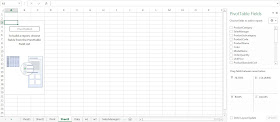
After you click OK, the blank PivotTable appears (Figure 6), ready for fields to be added to the report.
Fig. 6: Blank PivotTable with Fields on right side
From the right hand side in the PivotTable Fields, you can select the desired items to analyze and drag them to the appropriate quadrant in the bottom right corner, below the PivotTable Fields list. 

To produce a report regarding the total sales from 2005-2008 of categorized products sold under all sales managers, you select the ProductCategory, SalesManager, Year, and SalesAmount fields and drag them to the areas of rows for the first two, columns and values for the last two, as shown below in Figure 7.


Fig. 7: PivotTable with Sales of Products by Sales Managers by Year

There you have your PivotTable.

Thanks for reading,
Wayne