VLOOKUP
By opening the PivotTable workbook in Excel you can observe the relevant data for the fictional products of the example company, AdventureWorks. Figure 1 shows a segment of the data. |
| Fig. 1: AdventureWorks Sales data |
=VLOOKUP([@ProductCategory], SalesManagers, 2)The above VLOOKUP function matches the elements of the ProductCategory field of the current (Sales) sheet to first column of the SalesManager sheet, and retrieves the element of the corresponding second column (SalesManager) of the SalesManagers sheet. So, the Sales Manager of a specific product category shown on the SalesManagers sheet will be added to the respective category of product on the Sales sheet.
 |
| Fig. 2: VLOOKUP adding Sales Manager column in Sales sheet |
 |
| Fig. 3: SalesManagers sheet |
PivotTables
This information is stored as an Excel table. To make a PivotTable, which allows analysis of many fields, and later can be linked together into a data model, Excel requires PowerPivot to be enabled in Excel 2013, and downloaded and installed for Excel 2010. (Click here on how to enable PowerPivot in Excel versions 2013 or 2010.) When PowerPivot is enabled, you should see the PowerPivot displayed in Excel's ribbon tab at the top right (Figure 4).
| Fig. 4: PowerPivot tab in Excel 2013 |
 |
| Fig. 5: PivotTable options |
 |
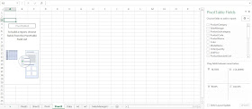
| Fig. 6: Blank PivotTable with Fields on right side |
To produce a report regarding the total sales from 2005-2008 of categorized products sold under all sales managers, you select the ProductCategory, SalesManager, Year, and SalesAmount fields and drag them to the areas of rows for the first two, columns and values for the last two, as shown below in Figure 7.
 |
| Fig. 7: PivotTable with Sales of Products by Sales Managers by Year |
There you have your PivotTable.
Thanks for reading,
Wayne
No comments:
Post a Comment