Pages

Wednesday, August 27, 2014

Natural Language Processing in Python: Part 2. Counting Vocabulary


Hello Readers,

Welcome to Part 2 of the Text Analysis with Python series. Here we will quantify words and tokens in texts with the nltk module in IPython. For more on getting started with nltk, click here.


Loading Texts

We start by load the texts we will be using from nltk.book. Remember to use "ipython" with "--matplotlib" in the command line to start. After we import the texts, we can see the titles in the output.

Code:
 1
 2
 3
 4
 5
 6
 7
 8
 9
10
11
12
13
14
15
16
17
18
19
20
21
22
23
24
25
26
27
28
29
30
31
Microsoft Windows [Version 6.1.7601]
Copyright (c) 2009 Microsoft Corporation.  All rights reserved.

C:\Users\wayne>ipython --matplotlib
Python 2.7.8 (default, Jun 30 2014, 16:03:49) [MSC v.1500 32 bit (Intel)]
Type "copyright", "credits" or "license" for more information.

IPython 2.1.0 -- An enhanced Interactive Python.
?         -> Introduction and overview of IPython's features.
%quickref -> Quick reference.
help      -> Python's own help system.
object?   -> Details about 'object', use 'object??' for extra details.
Using matplotlib backend: Qt4Agg

In [1]: from nltk.book import *
*** Introductory Examples for the NLTK Book ***
Loading text1, ..., text9 and sent1, ..., sent9
Type the name of the text or sentence to view it.
Type: 'texts()' or 'sents()' to list the materials.
text1: Moby Dick by Herman Melville 1851
text2: Sense and Sensibility by Jane Austen 1811
text3: The Book of Genesis
text4: Inaugural Address Corpus
text5: Chat Corpus
text6: Monty Python and the Holy Grail
text7: Wall Street Journal
text8: Personals Corpus
text9: The Man Who Was Thursday by G . K . Chesterton 1908

In [2]: text3
Out[2]: <Text: The Book of Genesis>

We will take a closer look at the third text, Book of Genesis.


Counting

First off, we start with the length of the text with "len()". It turns out that there are 44,764 tokens, or sequences of characters in text 3. Of course some words are used more than once. To obtain the unique tokens, we use "set()", and we nest it in "sorted()" to sort alphabetically. Looking at the first 20, we first observe punctuation, then our first word, "A", followed by "Abel". Note that after punctuation, capitalized words precede un-capitalized words in order.

Code:
 1
 2
 3
 4
 5
 6
 7
 8
 9
10
11
12
13
14
15
16
17
18
19
20
21
22
23
24
25
26
27
28
29
30
31
In [3]: len(text3)
Out[3]: 44764

# 44674 tokens
# token == name for sequence of characters
# for unique tokens, use set()

In [6]: sorted(set(text3))[:20]
Out[6]:
[u'!',
 u"'",
 u'(',
 u')',
 u',',
 u',)',
 u'.',
 u'.)',
 u':',
 u';',
 u';)',
 u'?',
 u'?)',
 u'A',
 u'Abel',
 u'Abelmizraim',
 u'Abidah',
 u'Abide',
 u'Abimael',
 u'Abimelech']

# punctuation and capital words precede lower case words


Distinct Count

For the number of unique tokens, we saw that "set()" would return an array of the tokens. To get a count, we just nest it in "len()".

Code:
1
2
3
4
5
6
7
8
In [7]: len(set(text3))
Out[7]: 2789

# has 2,789 distinct types
# word type =  form or spelling of word independent of its 
## specific occurrences in the text (unique)
# type = includes word types and punctuation
# which is why 2,789 is types not word types

Note that we include punctuation in the types as well since there are not word types only. We arrive at 2,789 distinct types used in text 3, Book of Genesis.


Lexical Diversity

Looking at a particular text, we can measure the average use of a word with the division of the total number of words by the number of unique ones. This measure will tell us the average number of times an average word is used. To create the measure we will take the "len()" and divide it by the "len(set()" of text 3. Note to import the division from __future__ to use floating point division, since Python versions 2.** uses integer division.

For text 3, we see that the average type is used roughly 16 times on average in the text. By using ".count()", we can numerate the occurrence of a sequence of characters. For example, "smote" in text 3 has 5 occurrences, less than the average of 16.

Code:
 1
 2
 3
 4
 5
 6
 7
 8
 9
10
11
12
13
14
15
16
17
18
19
20
21
22
23
24
25
26
27
28
29
30
31
32
# lexical richness of text

In [5]: from __future__ import division

In [6]: len(text3) / len(set(text3))
Out[6]: 16.050197203298673

In [7]: text3.count('smote')
Out[7]: 5

In [8]: 100*text4.count('a') / len(text4)
Out[8]: 1.4643016433938312

In [9]: texts()
text1: Moby Dick by Herman Melville 1851
text2: Sense and Sensibility by Jane Austen 1811
text3: The Book of Genesis
text4: Inaugural Address Corpus
text5: Chat Corpus
text6: Monty Python and the Holy Grail
text7: Wall Street Journal
text8: Personals Corpus
text9: The Man Who Was Thursday by G . K . Chesterton 1908

In [10]: text5.count('lol')
Out[10]: 704

In [11]: text5.count('lol')/len(text5)*100
Out[11]: 1.5640968673628082

In [12]: len(text5)/len(set(text5))
Out[12]: 7.420046158918563

When we take the count and divide it by the total types and multiply by 100, we get the percentage of that particular word in the text. So for an often used word such as 'a' in the fourth text, Inaugural Address Corpus, it occurs in ~1.46% of the text.


A text or internet short hand 'lol', for laugh out loud, occurs 704 times, at ~1.56% in text five, the chat room corpus. However, the diversity of words is quite high, as the average word is used only about 7.4 times, compared to higher repeats of 16 in text 3, the Book of Genesis.

So here we covered how to count words, determine the length of the text, find the number of distinct types, and word diversity in Python. Stay tuned for more posts!


Thanks for reading,

Wayne
@beyondvalence
LinkedIn

Text Analysis Series:
1. Natural Language Processing in Python: Part 1. Texts
2. Natural Language Processing in Python: Part 2. Counting Vocabulary
3. Natural Language Processing in Python: Part 3. Indexing Lists
4. Natural Language Processing in Python: Part 4. Frequency Distributions, Word Selections, & Collocations
.
Sunday, August 24, 2014

Earthquakes and USGS


Hello Readers,

Early Sunday morning on the 24th, there was an 6.0 magnitude earthquake which hit around 3:20 AM near the San Francisco Bay area by Napa and American Canyon. From the U.S. Geological Survey, we can find the earthquake information.

Here we will use Python (2.7.5) to retrieve and plot the magnitudes of recent recorded earthquakes by the USGS.


Using Python to Access USGS

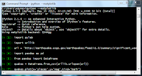
Opening the command prompt, start iPython with matplotlib module. It should look something like this:


Figure 1. iPython

Then we need to import urllib, and pylab for URL access and plotting, respectively. Using the ".urlopen()" method in urllib we will open the desired URL- the significant earthquakes in the past day, updated every 5 minutes as a CSV file (here).


Code:
 1
 2
 3
 4
 5
 6
 7
 8
 9
10
11
12
13
14
15
16
17
18
19
20
21
22
23
In [1]: import urllib

In [2]: url = 'http://earthquake.usgs.gov/earthquakes/feed/v1.0/summary/significant_week.csv'

In [3]: quakes = urllib.urlopen(url)

In [4]: for record in quakes:
   ...:     print(record)
   ...:

time,latitude,longitude,depth,mag,magType,nst,gap,dmin,rms,net,id,updated,place,type

2014-08-24T23:21:45.980Z,-14.5864,-73.5777,101,6.9,mww,,23,4.095,1.32,us,usb000s5x1,2014-08-25T00:50
:04.000Z,"43km ENE of Tambo, Peru",earthquake

2014-08-24T10:20:44.000Z,38.2202,-122.3128,11.3,6,Mw,146,28.8,0.03593261,0.16,nc,nc72282711,2014-08-
25T01:13:29.811Z,"6km NW of American Canyon, California",earthquake

2014-08-23T22:32:23.630Z,-32.7049,-71.3967,35,6.4,mww,,30,0.419,0.9,us,usb000s5rc,2014-08-24T11:48:3
9.000Z,"18km WNW of Hacienda La Calera, Chile",earthquake

2014-08-19T12:41:35.220Z,35.8186,-97.4718,3.46,4.2,mb,,29,0.025,0.69,us,usb000s45z,2014-08-24T06:27:
52.792Z,"7km SSW of Guthrie, Oklahoma",earthquake

We iterate through each line with "for" and print the all the records. As you can see, the first line is the header, containing the names of the columns. In the second set of earthquake information (3rd row), we spot the early morning earthquake in California.


Organizing into DataFrame

Since the rows are quite difficult to read, we can transform "quakes" into a DataFrame, using the ".from_csv()" method in DataFrame. It generates a tidy table from which we can view the data in the output below.

Code:
 1
 2
 3
 4
 5
 6
 7
 8
 9
10
11
12
13
14
15
16
17
18
19
20
21
22
23
24
25
26
27
28
29
30
31
32
33
34
35
36
37
In [5]: from pandas import DataFrame

In [6]: import pandas as pd

In [7]: quakes = urllib.urlopen(url)

In [8]: frame = DataFrame.from_csv(quakes)

In [9]: frame
Out[9]:
                            latitude  longitude   depth  mag magType  nst  \
time
2014-08-24 23:21:45.980000  -14.5864   -73.5777  101.00  6.9     mww  NaN
2014-08-24 10:20:44          38.2202  -122.3128   11.30  6.0      Mw  146
2014-08-23 22:32:23.630000  -32.7049   -71.3967   35.00  6.4     mww  NaN
2014-08-19 12:41:35.220000   35.8186   -97.4718    3.46  4.2      mb  NaN

                             gap      dmin   rms net          id  \
time
2014-08-24 23:21:45.980000  23.0  4.095000  1.32  us  usb000s5x1
2014-08-24 10:20:44         28.8  0.035933  0.16  nc  nc72282711
2014-08-23 22:32:23.630000  30.0  0.419000  0.90  us  usb000s5rc
2014-08-19 12:41:35.220000  29.0  0.025000  0.69  us  usb000s45z

                                             updated  \
time
2014-08-24 23:21:45.980000  2014-08-25T00:50:04.000Z
2014-08-24 10:20:44         2014-08-25T01:28:14.766Z
2014-08-23 22:32:23.630000  2014-08-24T11:48:39.000Z
2014-08-19 12:41:35.220000  2014-08-24T06:27:52.792Z

                                                            place        type
time
2014-08-24 23:21:45.980000                43km ENE of Tambo, Peru  earthquake
2014-08-24 10:20:44         6km NW of American Canyon, California  earthquake
2014-08-23 22:32:23.630000  18km WNW of Hacienda La Calera, Chile  earthquake
2014-08-19 12:41:35.220000           7km SSW of Guthrie, Oklahoma  earthquake

The 3:20 AM earthquake occured 6 kilometers North West of American Canyon in California  with a magnitude of 6.0 from the 'place' variable. More recently, there was another earthquake in Peru with a magnitude of 6.9.


Plotting Magnitude

We can compare the magnitudes by using the ".plot()" function. We specify the x-axis to be the 'place' and the y-axis to be the 'mag', or magnitude, and we want a horizontal bar plot through 'kind='barh''.

Code:
1
2
In [10]: frame.plot(x='place',y='mag',kind='barh')
Out[10]: <matplotlib.axes.AxesSubplot at 0x87682b0>
Figure 2. Plot of Earthquake Magnitudes


Great! That concludes this short post of using Python to retrieve CSV files from the USGS and basic plotting. Stay tuned for more posts!


Thanks for reading,

Wayne
@beyondvalence
LinkedIn

Thursday, August 21, 2014

Natural Language Processing in Python: Part 1. Texts


Hello Readers,

Here we begin exploring Natural Language Processing in Python using the nltk module. Previously, I posted a Text Mining blog series, specifically with Twitter data. With Python we progress one step further into Text Analysis: language processing.

Let us get started. Start up Python (I am using 2.7), and install the nltk module with "pip install nltk" from the command line or use the installer from their website.


Starting nltk

nltk consists of multiple lexical sources, corpora, or structured text, and text processing libraries. You first need to download the text sources using "import nltk" and "nltk.download()", after which a download box should appear. Choose the destination folder, select the book option in Collections, and click download.


Figure 1. nltk Download

To check the installation, "from nltk.book import *" would import all the books in the collection. In your command prompt, it might look similar to this:


Figure 2. IPython in the Command Prompt with nltk Books 

Note that it might take more than a few seconds for the large texts to load. Below (and above in Figure 2), you can view the loaded nine text names, and you can print them again with "texts()". To gather information about a specific text, just type in the text number, "text1", and it turns out to be Moby Dick written by Herman Melville in 1851.

Code:
 1
 2
 3
 4
 5
 6
 7
 8
 9
10
11
12
13
14
15
16
17
In [2]: from nltk.book import *
*** Introductory Examples for the NLTK Book ***
Loading text1, ..., text9 and sent1, ..., sent9
Type the name of the text or sentence to view it.
Type: 'texts()' or 'sents()' to list the materials.
text1: Moby Dick by Herman Melville 1851
text2: Sense and Sensibility by Jane Austen 1811
text3: The Book of Genesis
text4: Inaugural Address Corpus
text5: Chat Corpus
text6: Monty Python and the Holy Grail
text7: Wall Street Journal
text8: Personals Corpus
text9: The Man Who Was Thursday by G . K . Chesterton 1908

In [3]: text1
Out[3]: <Text: Moby Dick by Herman Melville 1851>

Looking through the texts, there are numerous variety among them. From Jane Austen, to the Book of Genesis, it provides quite a selection: the Inaugural Address Corpus, Chat Corpus, which covers uncensored chat room dialogue, and text from the Wall Street Journal. Typing the text key, such as "text1", will give more information about the text. 


Searching Text

Now that we have access to the text, we can begin exploring the contents. One useful method of the Text object is ".concordance()". It prints the context of a particular word where it occurs in the text. This is an excellent way to understand how the author uses a specific word. For example, we search for the word "monstrous" in the first text, Moby Dick below. The method returns 11 matches of the "monstrous" and also gives the words around where it occurs in the text.

Code:
 1
 2
 3
 4
 5
 6
 7
 8
 9
10
11
12
13
14
15
16
17
18
19
20
21
22
23
24
25
26
27
28
29
30
31
32
33
34
35
36
37
38
39
40
41
42
43
44
45
46
In [4]: text1.concordance('monstrous')
Building index...
Displaying 11 of 11 matches:
ong the former , one was of a most monstrous size . ... This came towards us ,
ON OF THE PSALMS . " Touching that monstrous bulk of the whale or ork we have r
ll over with a heathenish array of monstrous clubs and spears . Some were thick
d as you gazed , and wondered what monstrous cannibal and savage could ever hav
that has survived the flood ; most monstrous and most mountainous ! That Himmal
they might scout at Moby Dick as a monstrous fable , or still worse and more de
th of Radney .'" CHAPTER 55 Of the Monstrous Pictures of Whales . I shall ere l
ing Scenes . In connexion with the monstrous pictures of whales , I am strongly
ere to enter upon those still more monstrous stories of them which are to be fo
ght have been rummaged out of this monstrous cabinet there is no telling . But
of Whale - Bones ; for Whales of a monstrous size are oftentimes cast up dead u

In [5]: text2
Out[5]: <Text: Sense and Sensibility by Jane Austen 1811>

In [6]: text2.concordance('affection')
Building index...
Displaying 25 of 79 matches:
, however , and , as a mark of his affection for the three girls , he left them
t . It was very well known that no affection was ever supposed to exist between
deration of politeness or maternal affection on the side of the former , the tw
d the suspicion -- the hope of his affection for me may warrant , without impru
hich forbade the indulgence of his affection . She knew that his mother neither
rd she gave one with still greater affection . Though her late conversation wit
 can never hope to feel or inspire affection again , and if her home be uncomfo
m of the sense , elegance , mutual affection , and domestic comfort of the fami
, and which recommended him to her affection beyond every thing else . His soci
ween the parties might forward the affection of Mr . Willoughby , an equally st
 the most pointed assurance of her affection . Elinor could not be surprised at
he natural consequence of a strong affection in a young and ardent mind . This
 opinion . But by an appeal to her affection for her mother , by representing t
 every alteration of a place which affection had established as perfect with hi
e will always have one claim of my affection , which no other can possibly shar
f the evening declared at once his affection and happiness . " Shall we see you
ause he took leave of us with less affection than his usual behaviour has shewn
ness ." " I want no proof of their affection ," said Elinor ; " but of their en
onths , without telling her of his affection ;-- that they should part without
ould be the natural result of your affection for her . She used to be all unres
distinguished Elinor by no mark of affection . Marianne saw and listened with i
th no inclination for expense , no affection for strangers , no profession , an
till distinguished her by the same affection which once she had felt no doubt o
al of her confidence in Edward ' s affection , to the remembrance of every mark
 was made ? Had he never owned his affection to yourself ?" " Oh , no ; but if

Additionally, we can search the second text, Jane Austen's Sense and Sensibility for the word "affection". ".concordance()" returns the first 25 matches from the total 79 in the text, while showing the word context.


What about the similarities among contexts of a certain word? We would use ".similar()" and it would show us the similar context words from our ".concordance()" output. For the word 'monstrous', in text1, some words used in the same context are : "imperial", "subtly", "impalpable", etc. In Moby Dick, Melville uses 'monstrous' quite differently when compared to 'monstrous' in Sense and Sensibility by Austen.


Code:

 1
 2
 3
 4
 5
 6
 7
 8
 9
10
11
12
13
In [9]: text1.similar('monstrous')
Building word-context index...
imperial subtly impalpable pitiable curious abundant perilous
trustworthy untoward singular lamentable few determined maddens
horrible tyrannical lazy mystifying christian exasperate

In [10]: text2.similar('monstrous')
Building word-context index...
a great good very amazingly exceedingly as so sweet heartily
remarkably extremely vast

In [12]: text2.common_contexts(['monstrous','very'])
a_pretty is_pretty a_lucky am_glad be_glad

Austen uses 'monstrous' with words such as 'great', 'good', 'amazingly', and 'sweet'. Therefore, Melville writes 'monstrous' with sometimes a positive or negative connotation, whereas Austen associates 'monstrous' with a positive connotation in Sense and Sensibility. You can also see the similar context words for two words with the ".common_contexts()" method. The words 'monstrous' and 'very' are belong in the same group as 'pretty', 'lucky', and 'glad', all positive adjectives.


Inaugural Address Corpus

Now we move on to the large corpus composed of Presidential inaugural addresses. Looking at a keyword such as 'freedom', ".concordance()" prints the first 25 of 183. Many of the early mentions have the structure: "freedom of ___", where blank is religion the press, etc. 

Code:
 1
 2
 3
 4
 5
 6
 7
 8
 9
10
11
12
13
14
15
16
17
18
19
20
21
22
23
24
25
26
27
28
29
30
31
32
33
34
35
36
37
38
39
40
In [14]: text4
Out[14]: <Text: Inaugural Address Corpus>

In [15]: text4.concordance('freedom')
Building index...
Displaying 25 of 183 matches:
s at the bar of the public reason ; freedom of religion ; freedom of the press
blic reason ; freedom of religion ; freedom of the press , and freedom of perso
ligion ; freedom of the press , and freedom of person under the protection of t
e instrumental to the happiness and freedom of all . Relying , then , on the pa
s of an institution so important to freedom and science are deeply to be regret
 be fairly and fully made , whether freedom of discussion , unaided by power ,
te and personal rights , and of the freedom of the press ; to observe economy i
rdinary lot of humanity secured the freedom and happiness of this people . We n
s inseparable from the enjoyment of freedom , but which have more than once app
 the abuse of power consists in the freedom , the purity , and the frequency of
ation to the civil power ; that the freedom of the press and of religious opini
 own ; to cherish the principles of freedom and of equal rights wherever they w
l Government into conflict with the freedom of elections , and the counteractio
f appointment more independence and freedom from such influences might be expec
e it might exert in controlling the freedom of the elective franchise . If such
of the Executive in controlling the freedom of the elective franchise through t
 from the mother country that " the freedom of the press is the great bulwark o
the people as the genuine spirit of freedom , and , like the false Christs whos
by the gifts of civil and religious freedom , who watched over and prospered th
 , which have been the offspring of freedom , and not of power . This most admi
ween church and state , and perfect freedom of opinion is guaranteed to all sec
o circumscribed the limits of human freedom and planted their standard , where
encouragement and potent appeal for freedom will be its own history -- its tria
ur sympathies in the cause of human freedom and universal advancement . But the
this Constitution the boundaries of freedom have been enlarged , the foundation

In [16]: text4.similar('freedom')
Building word-context index...
aided practicability dissolution all obstruction protest aegis
integrity assembled aggression votes paris boastfulness refunding
impoverishment under pride merchant lure risk

In [17]: text4.common_contexts(['freedom','terror'])
of_and the_of of_that

What do the contexts of 'freedom' have in common with each other? Again, with ".similar()" we see "aided", "practicability", "dissolution", "all", "obstruction", and many other terms. What about the contexts of 'freedom' and 'terror'? With the recent War on Terror, do any of the word choices reflect the events of the times? Not really, with words "of", "and", "the", and "that", it appears that those two words do not use similar words when spoken in an address.


Dispersion Plot


Since the Inaugural Address Corpus contains addresses from over the years, we can use a dispersion plot to uncover any temporal trends in word usage. With ".dispersion_plot()" we pass an array of terms which we want to visualize. Let's look at the terms 'citizens', 'democracy', 'freedom', 'duties', and 'America'.

Code:
1
In [19]: text4.dispersion_plot(['citizens','democracy','freedom','duties','America'])

The result is this plot:


Figure 3. Dispersion Plot, Text4


We can see that 'citizens' is best distributed, therefore, most used through the years in addresses. 'freedom' and 'America' see quick increases in usage around the 80,000 word offset. More addresses contain 'freedom' and 'America', while less addresses contain the word 'duties' in recent years when compared to earlier addresses. This could be explained by the World Wars and the emergence of the US as a subsequent world power- where fighting for 'freedom' and 'America' were relevant political keywords. We can see that some words call into favor while others, such as 'duties', fall from favor.


Okay folks, you have just read a post on natural language processing using the nltk module in Python. You learned how to search for word contexts, compare the contexts, and find similar words with different word contexts. Also, when the text is organized by time, we can use the dispersion plot to visualize word frequency and usage by time. Stay tuned for the next post in this series!


Thanks for reading,

Wayne
@beyondvalence
LinkedIn

Text Analysis Series:
1. Natural Language Processing in Python: Part 1. Texts
2. Natural Language Processing in Python: Part 2. Counting Vocabulary
3. Natural Language Processing in Python: Part 3. Indexing Lists
4. Natural Language Processing in Python: Part 4. Frequency Distributions, Word Selections, & Collocations
.

Monday, August 18, 2014

Python and Pandas: Part 1. bit.ly and Time Zones


Hello Readers,

Here we will explore analytics with Python and Pandas by looking at URL data shortened by bit.ly. In 2011, the United States government partnered with bit.ly to provide anonymous data on users who shortened links ending with .gov or .mil. You can find the data here.

I will be using Python 2.7.5 with sci-kit-learn, and the bit.ly data from March 16th, 2012. We aim to quantify and plot the top time zones in the dataset.


Reading the Data

Start the command prompt and navigate to the directory where you saved the text file. Assuming you installed the libraries correctly, typing "ipython notebook --pylab=inline" will start Python in that directory with the data file:


Figure 1. IPython Command Prompt
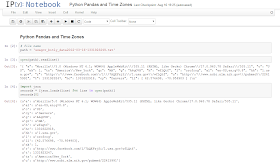
Make sure you navigate to the specific directory where the data is located, but you cal also click to navigate after IPython is launched. For this post, the code and results in IPython look like Figure 2 in your web browser (I am using Chrome). More on IPython can be found here. Essentially, cells containing code that can be executed sequentially, with the results being printed below each cell.


Figure 2. IPython Notebook

Here is the code below. We start by specifying the file name, and reading the first line with ".readline()". Immediately we realize that it is formatted, likely to be JSON. So we import the json module, and use the method "json.loads()" to format each line read by "open()" into "records". Looking at the first "record[0]", we observe the key:value pairs, verifying it is indeed in JSON format.


Code:

 1
 2
 3
 4
 5
 6
 7
 8
 9
10
11
12
13
14
15
16
17
18
19
20
21
22
23
24
25
26
27
28
29
30
31
32
33
34
35
# data file name
>>> path = 'usagov_bitly_data2012-03-16-1331923249.txt'
# read first line
>>> open(path).readline()

'{ "a": "Mozilla\\/5.0 (Windows NT 6.1; WOW64) AppleWebKit\\/535.11 (KHTML, like Gecko) Chrome\\/17.0.963.78 Safari\\/535.11", "c": "US", "nk": 1, "tz": "America\\/New_York", "gr": "MA", "g": "A6qOVH", "h": "wfLQtf", "l": "orofrog", "al": "en-US,en;q=0.8", "hh": "1.usa.gov", "r": "http:\\/\\/www.facebook.com\\/l\\/7AQEFzjSi\\/1.usa.gov\\/wfLQtf", "u": "http:\\/\\/www.ncbi.nlm.nih.gov\\/pubmed\\/22415991", "t": 1331923247, "hc": 1331822918, "cy": "Danvers", "ll": [ 42.576698, -70.954903 ] }\n'

# use json format
>>> import json
# format json by each line
# into key:value pairs
>>> records = [json.loads(line) for line in open(path)]
>>> records[0]

{u'a': u'Mozilla/5.0 (Windows NT 6.1; WOW64) AppleWebKit/535.11 (KHTML, like Gecko) Chrome/17.0.963.78 Safari/535.11',
 u'al': u'en-US,en;q=0.8',
 u'c': u'US',
 u'cy': u'Danvers',
 u'g': u'A6qOVH',
 u'gr': u'MA',
 u'h': u'wfLQtf',
 u'hc': 1331822918,
 u'hh': u'1.usa.gov',
 u'l': u'orofrog',
 u'll': [42.576698, -70.954903],
 u'nk': 1,
 u'r': u'http://www.facebook.com/l/7AQEFzjSi/1.usa.gov/wfLQtf',
 u't': 1331923247,
 u'tz': u'America/New_York',
 u'u': u'http://www.ncbi.nlm.nih.gov/pubmed/22415991'}

# first record with value in time zone key
>>> records[0]['tz']

u'America/New_York'

Additionally, we can take the first record and looking at specific keys, such as the time zone key "tz". So on March 16th, the first computer user used bit.ly to shorten a .gov or .mil URL from "u'
America/New_York'".

Great, now that we have located the time zone locations in the data, we can proceed with analyzing those key:value pairs.


pandas

Through the pandas module, we work with the data structure "DataFrame", similar to the data.frame object in R. We simply use the method "DataFrame()" to turn our "records" into a DataFrame object, consisting of entries (rows) and data columns. By calling "frame['tz'][:10]", we take the first 10 entries from the time zone column. Note the blank entries in the output. Entries 7, 8, and 9 do not have a location. Therefore we need to deal with missing data. 

Use the ".fillna()" method to replace the NA values with a string, such as 'missing', and the blank values "clean_tz == '' " with 'unknown'. Now we utilize the ".value_counts()" method to create the counts of the time zones in "tz_counts".

Code:
 1
 2
 3
 4
 5
 6
 7
 8
 9
10
11
12
13
14
15
16
17
18
19
20
21
22
23
24
25
26
27
28
29
30
31
32
33
34
35
36
37
38
39
40
41
42
43
44
# use pandas
>>> from pandas import DataFrame, Series
>>> import pandas as pd
# convert to DataFrame
>>> frame = DataFrame(records)
# first 10 in column 'tz' 
>>> frame['tz'][:10]

0     America/New_York
1       America/Denver
2     America/New_York
3    America/Sao_Paulo
4     America/New_York
5     America/New_York
6        Europe/Warsaw
7                     
8                     
9                     
Name: tz, dtype: object

# need to find the NAs and blanks
>>> clean_tz = frame['tz'].fillna('missing')
>>> clean_tz[clean_tz == ''] = 'unknown'

# use value_counts() method
>>> tz_counts = clean_tz.value_counts()
# first 10 labeled correctly
>>> tz_counts[:10]

America/New_York       1251
unknown                 521
America/Chicago         400
America/Los_Angeles     382
America/Denver          191
missing                 120
Europe/London            74
Asia/Tokyo               37
Pacific/Honolulu         36
Europe/Madrid            35
dtype: int64

# plot top 10
>>> tz_counts[:10].plot(kind='barh',rot=0)
 

Taking the first 10 time zones, we see they are ordered by high to low frequency. "America/New_York" was the more frequent, with 1,251 counts, followed by 521 "unknown" values, and 400 "America/Chicago".


Lastly, we can use the ".plot()" method to create a plot of the time zone counts. The plot method is made available when we issued the argument in the command line with "--pylab=inline".


Figure 3. Top Time Zone Frequencies

Clearly New York took the top spot, with the most bit.ly government URL usage. But that is not all. We can look at more variables, such as the agent.


Plotting by Agent


The Data column 'a' stands for the agent which accessed the bit.ly services from the computer. It could have been Mozilla Firefox, Safari, Google Chrome, etc. We can stratify the time zones by agent to see any differences in agent usage by time zone.


To do this, we need to parse the string value in 'a' with ".split()". The first five results show Mozilla 5.0 and 4.0, and Google Maps from Rochester. Again using the ".value_counts()" method, we quantify the top 8 agents in "results". The top three were Mozilla 5.0 and 4.0, and Google Maps Rochester NY, respectively.


Code:
 1
 2
 3
 4
 5
 6
 7
 8
 9
10
11
12
13
14
15
16
17
18
19
20
21
22
23
24
25
26
27
28
29
30
31
32
33
34
35
36
37
38
39
40
41
42
43
44
45
46
47
48
49
50
51
52
53
54
55
# find 'a' agent
>>> results = Series([x.split()[0] for x in frame.a.dropna()])
>>> results[:5]

0               Mozilla/5.0
1    GoogleMaps/RochesterNY
2               Mozilla/4.0
3               Mozilla/5.0
4               Mozilla/5.0
dtype: object

>>> results.value_counts()[:8]

Mozilla/5.0                 2594
Mozilla/4.0                  601
GoogleMaps/RochesterNY       121
Opera/9.80                    34
TEST_INTERNET_AGENT           24
GoogleProducer                21
Mozilla/6.0                    5
BlackBerry8520/5.0.0.681       4
dtype: int64

>>> # decompose time zones into Windows and non-Windows users
>>> # use 'a' agent string to find 'Windows'
>>> cframe = frame[frame.a.notnull()]
>>> os = np.where(cframe['a'].str.contains('Windows'), 'Windows', 'Not Windows')
>>> os[:5]

0        Windows
1    Not Windows
2        Windows
3    Not Windows
4        Windows
Name: a, dtype: object

>>> # group data by time zone and operating systems
>>> by_tz_os = cframe.groupby(['tz', os])
>>> # group counts calculated by size
>>> agg_counts = by_tz_os.size().unstack().fillna(0)
>>> agg_counts[:10]

a      Not Windows Windows
tz  
      245  276
Africa/Cairo     0  3
Africa/Casablanca    0  1
Africa/Ceuta     0  2
Africa/Johannesburg    0  1
Africa/Lusaka     0  1
America/Anchorage    4  1
America/Argentina/Buenos_Aires                 1  0
America/Argentina/Cordoba          0  1
America/Argentina/Mendoza          0  1
 

How would we find the Windows and non-Windows users? Well, we take a non-null subset of "frame" and find if the value in 'a' contains 'Windows' or not, via ".str.contains('Windows')". If true, the we label it 'Windows', else, 'Not Windows'. Peering into the first 5 entries in "os", the first entry has 'Windows', whereas the second is 'Not Windows'.


To aggregate the time zones and agents, we use the ".groupby()" method, specifying "['tz', os]" for the values. Looking at the first 10, cleaned with ".size().unstack().fillna(0)", we see blank values followed by "Africa/Cairo", "Africa/Casablanca", etc. grouped by Windows.

To gather an order of the frequent time zones, we first sort out an index by summing across the rows using ".sum(1).argsort()". So now the 'tz' time zones have an index by count. Then we use the index to order the counts into "count_subset" using ".take(indexer)". The "[-10:]" means we take the 10 entries starting from the last entry, so the last 10.


Code:
 1
 2
 3
 4
 5
 6
 7
 8
 9
10
11
12
13
14
15
16
17
18
19
20
21
22
23
24
25
26
27
28
29
30
31
32
33
34
35
36
37
38
39
40
41
42
43
44
>>> # top over-all time zones?
>>> # construct indirect index array from row counts
>>> indexer = agg_counts.sum(1).argsort()
>>> indexer[:10]

tz
                                  24
Africa/Cairo                      20
Africa/Casablanca                 21
Africa/Ceuta                      92
Africa/Johannesburg               87
Africa/Lusaka                     53
America/Anchorage                 54
America/Argentina/Buenos_Aires    57
America/Argentina/Cordoba         26
America/Argentina/Mendoza         55
dtype: int64

>>> # use index as sort order
>>> count_subset = agg_counts.take(indexer)[-10:]
>>> count_subset


a    Not Windows         Windows
tz  
America/Sao_Paulo  13   20
Europe/Madrid   16   19
Pacific/Honolulu  0   36
Asia/Tokyo   2   35
Europe/London   43   31
America/Denver   132   59
America/Los_Angeles  130   252
America/Chicago   115   285
    245   276
America/New_York  339   912

>>> # visualize using stacked barplot
>>> count_subset.plot(kind='barh', stacked=True)
<matplotlib.axes.AxesSubplot at 0x890cd90>

>>> # normalizing the plot to percentage
>>> normed_subset = count_subset.div(count_subset.sum(1), axis=0)
>>> normed_subset.plot(kind='barh',stacked=True)
<matplotlib.axes.AxesSubplot at 0x8871c30>

Indeed, the table mirrors Figure 3, where we took the total entries of each time zone. Here we split each time zone into Windows/Not Windows, but they still add up to the same total for each time zone. We can see the totals by the ".plot()" method with "stacked=True", of each time zone, but also by each operating system within each time zone.


Figure 4. Windows Usage by Time Zone

For lower values, the Windows/Not Windows ratio cannot be seen easily, so we normalize to 1, thus forcing a percentage rather than raw counts. This way, each time zone can be compared with each other. This is done with ".div(count_subset.sum(1), axis=0)". So unlike Figure 4 where we see the absolute counts, Figure 5 features all counts forced to one, but split by proportion of Windows/Not Windows in green/blue.


Figure 5. Normalized Windows Usage by Time Zone

While New York might have the highest count, among the top time zones, Honolulu had the highest proportion of Windows agents, whereas Denver had the highest percentage of non-Windows agents using bit.ly.


I hope this post shows you how powerful Python is when the pandas module is used. Although Python still lags behind R as the statistical package of choice, it is catching up quickly. Additionally, Python is excellent for coding tasks other than statistical usage- so look out when programmers do not need to use R for their statistical analyses.


Thanks for reading,

Wayne
@beyondvalence
LinkedIn

Python and Pandas Series:
1. Python and Pandas: Part 1: bit.ly and Time Zones
2. Python and Pandas: Part 2. Movie Ratings
3. Python and Pandas: Part 3. Baby Names, 1880-2010
4. Python and Pandas: Part 4. More Baby Names