Python and Pandas: Part 1. bit.ly and Time Zones

Hello Readers,

Here we will explore analytics with Python and Pandas by looking at URL data shortened by bit.ly. In 2011, the United States government partnered with bit.ly to provide anonymous data on users who shortened links ending with .gov or .mil. You can find the data here.

I will be using Python 2.7.5 with sci-kit-learn, and the bit.ly data from March 16th, 2012. We aim to quantify and plot the top time zones in the dataset.

Reading the Data

Start the command prompt and navigate to the directory where you saved the text file. Assuming you installed the libraries correctly, typing "ipython notebook --pylab=inline" will start Python in that directory with the data file:

Figure 1. IPython Command Prompt

Make sure you navigate to the specific directory where the data is located, but you cal also click to navigate after IPython is launched. For this post, the code and results in IPython look like Figure 2 in your web browser (I am using Chrome). More on IPython can be found here. Essentially, cells containing code that can be executed sequentially, with the results being printed below each cell.

Figure 2. IPython Notebook

Here is the code below. We start by specifying the file name, and reading the first line with ".readline()". Immediately we realize that it is formatted, likely to be JSON. So we import the json module, and use the method "json.loads()" to format each line read by "open()" into "records". Looking at the first "record[0]", we observe the key:value pairs, verifying it is indeed in JSON format.

Code:

1 2 3 4 5 6 7 8 9 10 11 12 13 14 15 16 17 18 19 20 21 22 23 24 25 26 27 28 29 30 31 32 33 34 35

# data file name >>> path = 'usagov_bitly_data2012-03-16-1331923249.txt' # read first line >>> open(path).readline() '{ "a": "Mozilla\\/5.0 (Windows NT 6.1; WOW64) AppleWebKit\\/535.11 (KHTML, like Gecko) Chrome\\/17.0.963.78 Safari\\/535.11", "c": "US", "nk": 1, "tz": "America\\/New_York", "gr": "MA", "g": "A6qOVH", "h": "wfLQtf", "l": "orofrog", "al": "en-US,en;q=0.8", "hh": "1.usa.gov", "r": "http:\\/\\/www.facebook.com\\/l\\/7AQEFzjSi\\/1.usa.gov\\/wfLQtf", "u": "http:\\/\\/www.ncbi.nlm.nih.gov\\/pubmed\\/22415991", "t": 1331923247, "hc": 1331822918, "cy": "Danvers", "ll": [ 42.576698, -70.954903 ] }\n' # use json format >>> import json # format json by each line # into key:value pairs >>> records = [json.loads(line) for line in open(path)] >>> records[0] {u'a': u'Mozilla/5.0 (Windows NT 6.1; WOW64) AppleWebKit/535.11 (KHTML, like Gecko) Chrome/17.0.963.78 Safari/535.11', u'al': u'en-US,en;q=0.8', u'c': u'US', u'cy': u'Danvers', u'g': u'A6qOVH', u'gr': u'MA', u'h': u'wfLQtf', u'hc': 1331822918, u'hh': u'1.usa.gov', u'l': u'orofrog', u'll': [42.576698, -70.954903], u'nk': 1, u'r': u'http://www.facebook.com/l/7AQEFzjSi/1.usa.gov/wfLQtf', u't': 1331923247, u'tz': u'America/New_York', u'u': u'http://www.ncbi.nlm.nih.gov/pubmed/22415991'} # first record with value in time zone key >>> records[0]['tz'] u'America/New_York'

Additionally, we can take the first record and looking at specific keys, such as the time zone key "tz". So on March 16th, the first computer user used bit.ly to shorten a .gov or .mil URL from "u'America/New_York'".

Great, now that we have located the time zone locations in the data, we can proceed with analyzing those key:value pairs.

pandas

Through the pandas module, we work with the data structure "DataFrame", similar to the data.frame object in R. We simply use the method "DataFrame()" to turn our "records" into a DataFrame object, consisting of entries (rows) and data columns. By calling "frame['tz'][:10]", we take the first 10 entries from the time zone column. Note the blank entries in the output. Entries 7, 8, and 9 do not have a location. Therefore we need to deal with missing data. 

Use the ".fillna()" method to replace the NA values with a string, such as 'missing', and the blank values "clean_tz == '' " with 'unknown'. Now we utilize the ".value_counts()" method to create the counts of the time zones in "tz_counts".

Code:

1 2 3 4 5 6 7 8 9 10 11 12 13 14 15 16 17 18 19 20 21 22 23 24 25 26 27 28 29 30 31 32 33 34 35 36 37 38 39 40 41 42 43 44

# use pandas >>> from pandas import DataFrame, Series >>> import pandas as pd # convert to DataFrame >>> frame = DataFrame(records) # first 10 in column 'tz' >>> frame['tz'][:10] 0 America/New_York 1 America/Denver 2 America/New_York 3 America/Sao_Paulo 4 America/New_York 5 America/New_York 6 Europe/Warsaw 7 8 9 Name: tz, dtype: object # need to find the NAs and blanks >>> clean_tz = frame['tz'].fillna('missing') >>> clean_tz[clean_tz == ''] = 'unknown' # use value_counts() method >>> tz_counts = clean_tz.value_counts() # first 10 labeled correctly >>> tz_counts[:10] America/New_York 1251 unknown 521 America/Chicago 400 America/Los_Angeles 382 America/Denver 191 missing 120 Europe/London 74 Asia/Tokyo 37 Pacific/Honolulu 36 Europe/Madrid 35 dtype: int64 # plot top 10 >>> tz_counts[:10].plot(kind='barh',rot=0)

Taking the first 10 time zones, we see they are ordered by high to low frequency. "America/New_York" was the more frequent, with 1,251 counts, followed by 521 "unknown" values, and 400 "America/Chicago".

Lastly, we can use the ".plot()" method to create a plot of the time zone counts. The plot method is made available when we issued the argument in the command line with "--pylab=inline".

Figure 3. Top Time Zone Frequencies

Clearly New York took the top spot, with the most bit.ly government URL usage. But that is not all. We can look at more variables, such as the agent.

Plotting by Agent

The Data column 'a' stands for the agent which accessed the bit.ly services from the computer. It could have been Mozilla Firefox, Safari, Google Chrome, etc. We can stratify the time zones by agent to see any differences in agent usage by time zone.

To do this, we need to parse the string value in 'a' with ".split()". The first five results show Mozilla 5.0 and 4.0, and Google Maps from Rochester. Again using the ".value_counts()" method, we quantify the top 8 agents in "results". The top three were Mozilla 5.0 and 4.0, and Google Maps Rochester NY, respectively.

Code:

1 2 3 4 5 6 7 8 9 10 11 12 13 14 15 16 17 18 19 20 21 22 23 24 25 26 27 28 29 30 31 32 33 34 35 36 37 38 39 40 41 42 43 44 45 46 47 48 49 50 51 52 53 54 55

# find 'a' agent >>> results = Series([x.split()[0] for x in frame.a.dropna()]) >>> results[:5] 0 Mozilla/5.0 1 GoogleMaps/RochesterNY 2 Mozilla/4.0 3 Mozilla/5.0 4 Mozilla/5.0 dtype: object >>> results.value_counts()[:8] Mozilla/5.0 2594 Mozilla/4.0 601 GoogleMaps/RochesterNY 121 Opera/9.80 34 TEST_INTERNET_AGENT 24 GoogleProducer 21 Mozilla/6.0 5 BlackBerry8520/5.0.0.681 4 dtype: int64 >>> # decompose time zones into Windows and non-Windows users >>> # use 'a' agent string to find 'Windows' >>> cframe = frame[frame.a.notnull()] >>> os = np.where(cframe['a'].str.contains('Windows'), 'Windows', 'Not Windows') >>> os[:5] 0 Windows 1 Not Windows 2 Windows 3 Not Windows 4 Windows Name: a, dtype: object >>> # group data by time zone and operating systems >>> by_tz_os = cframe.groupby(['tz', os]) >>> # group counts calculated by size >>> agg_counts = by_tz_os.size().unstack().fillna(0) >>> agg_counts[:10] a Not Windows Windows tz 245 276 Africa/Cairo 0 3 Africa/Casablanca 0 1 Africa/Ceuta 0 2 Africa/Johannesburg 0 1 Africa/Lusaka 0 1 America/Anchorage 4 1 America/Argentina/Buenos_Aires 1 0 America/Argentina/Cordoba 0 1 America/Argentina/Mendoza 0 1

How would we find the Windows and non-Windows users? Well, we take a non-null subset of "frame" and find if the value in 'a' contains 'Windows' or not, via ".str.contains('Windows')". If true, the we label it 'Windows', else, 'Not Windows'. Peering into the first 5 entries in "os", the first entry has 'Windows', whereas the second is 'Not Windows'.

To aggregate the time zones and agents, we use the ".groupby()" method, specifying "['tz', os]" for the values. Looking at the first 10, cleaned with ".size().unstack().fillna(0)", we see blank values followed by "Africa/Cairo", "Africa/Casablanca", etc. grouped by Windows.

To gather an order of the frequent time zones, we first sort out an index by summing across the rows using ".sum(1).argsort()". So now the 'tz' time zones have an index by count. Then we use the index to order the counts into "count_subset" using ".take(indexer)". The "[-10:]" means we take the 10 entries starting from the last entry, so the last 10.

Code:

1 2 3 4 5 6 7 8 9 10 11 12 13 14 15 16 17 18 19 20 21 22 23 24 25 26 27 28 29 30 31 32 33 34 35 36 37 38 39 40 41 42 43 44

>>> # top over-all time zones? >>> # construct indirect index array from row counts >>> indexer = agg_counts.sum(1).argsort() >>> indexer[:10] tz 24 Africa/Cairo 20 Africa/Casablanca 21 Africa/Ceuta 92 Africa/Johannesburg 87 Africa/Lusaka 53 America/Anchorage 54 America/Argentina/Buenos_Aires 57 America/Argentina/Cordoba 26 America/Argentina/Mendoza 55 dtype: int64 >>> # use index as sort order >>> count_subset = agg_counts.take(indexer)[-10:] >>> count_subset a Not Windows Windows tz America/Sao_Paulo 13 20 Europe/Madrid 16 19 Pacific/Honolulu 0 36 Asia/Tokyo 2 35 Europe/London 43 31 America/Denver 132 59 America/Los_Angeles 130 252 America/Chicago 115 285 245 276 America/New_York 339 912 >>> # visualize using stacked barplot >>> count_subset.plot(kind='barh', stacked=True) <matplotlib.axes.AxesSubplot at 0x890cd90> >>> # normalizing the plot to percentage >>> normed_subset = count_subset.div(count_subset.sum(1), axis=0) >>> normed_subset.plot(kind='barh',stacked=True) <matplotlib.axes.AxesSubplot at 0x8871c30>

Indeed, the table mirrors Figure 3, where we took the total entries of each time zone. Here we split each time zone into Windows/Not Windows, but they still add up to the same total for each time zone. We can see the totals by the ".plot()" method with "stacked=True", of each time zone, but also by each operating system within each time zone.

Figure 4. Windows Usage by Time Zone

For lower values, the Windows/Not Windows ratio cannot be seen easily, so we normalize to 1, thus forcing a percentage rather than raw counts. This way, each time zone can be compared with each other. This is done with ".div(count_subset.sum(1), axis=0)". So unlike Figure 4 where we see the absolute counts, Figure 5 features all counts forced to one, but split by proportion of Windows/Not Windows in green/blue.

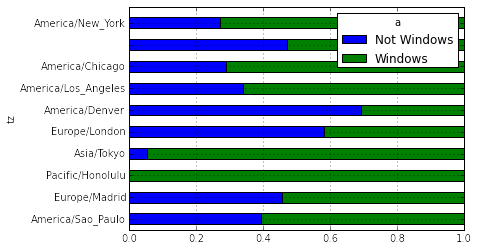Figure 5. Normalized Windows Usage by Time Zone

While New York might have the highest count, among the top time zones, Honolulu had the highest proportion of Windows agents, whereas Denver had the highest percentage of non-Windows agents using bit.ly.

I hope this post shows you how powerful Python is when the pandas module is used. Although Python still lags behind R as the statistical package of choice, it is catching up quickly. Additionally, Python is excellent for coding tasks other than statistical usage- so look out when programmers do not need to use R for their statistical analyses.



Thanks for reading,

Wayne
@beyondvalence
LinkedIn

Python and Pandas Series:
1. Python and Pandas: Part 1: bit.ly and Time Zones
2. Python and Pandas: Part 2. Movie Ratings
3. Python and Pandas: Part 3. Baby Names, 1880-2010
4. Python and Pandas: Part 4. More Baby Names
.