Hello Readers,

Today we continue our discussion about regression in QSAR modeling and venture into robust regression and estimating the performance of the model using cross-validation. Using the chemical solubility data set from the QSAR post, we will explore more regression topics!
Let us start R and begin!
Robust Regression
In the previous regression post we talked about ordinary regression with multiple (chemical descriptor) predictors trying to model compound solubility. Again, we require the following R packages: MASS, caret, AppliedPredictiveModeling, lars, pls, and elasticnet.
 |
| R Packages |
While using the Box-Cox transformed continuous variables in solTrainXtrans data set, we can perform robust regression with the rlm() function from MASS, similar to the lm() regression function in the last post. By default, the rlm() function uses the Huber approach to account for values which excessively influence the model by taking the sum of the differences instead of the sum of squared differences (SSE) above a threshold.
 |
| Robust Regression |
Because there are so many predictors, the results are truncated to show the beginning and the end, where all types of predictors are shown.
 |
| End of Robust Regression |
As we can see from the results above, the residual standard error was 0.3739. Previously, from the ordinary regression model, our RMSE was 0.5524, with the test prediction RMSE of 0.7456. Clearly we can see the difference from the two regression models, with the robust RMSE lower than the RMSE of the ordinary regression. Why? Because robust regression took into account larger residuals above a threshold and took the simple residual (difference), while using the squared residuals for smaller residuals. That is why we a smaller RMSE for the robust regression- it is more resistance to influential outliers.
Plotting the Predicted Values
We can visualize the robust regression results by using a plot of the predicted and true solubility values using predict() and plot().
| Predicting rlm and Plotting Predicted Solubilities |
Using the graph, we can compare the predicted values of the robust regression with those from the ordinary regression from the previous post by adding them as points() and creating a legend() to differentiate the two.
| Adding Predicted Regression Solubilities and Legend |
Which will yield us the graphic below:
As we can see, the two are very similar in distribution, while some predicted points between the two regression models vary.
Estimation of Model Performance
One method of evaluating how well the regression model fit an independent data set is through cross-validation, where we resample the entire data set in parts for the regression training. In other words, how well will the predictive model perform on an unknown data set? That is where cross-validation -a method of resampling- comes to our aid.
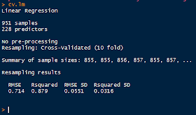
Using the trainControl() function, we can specify the type of resampling to be cross-validation with method="cv". Then with the train() function we input the predictor variables and response variable, and the resampling method is used as the type of control in trControl=ctrl.
| Cross-Validation Regression |
The subsequent summary is displayed below in three parts:
 |
| Cross-Validation Object |
 |
| Cross-Validation Summary Top |
 |
| Cross-Validation Continuous Variables |
And we conclude this post, folks! Here we compared robust regression and ordinary regression and saw (through the RMSE) how robust regression handled influential observations through the Huber function by taking the residual rather than the squared residual. Additionally we looked at predictive model performance through cross-validation and how we can determine how well a model will perform in practice on an unknown test set.
Stay tuned for more R and regression topics!
As always, thanks for reading!
Wayne
@beyondvalence

No comments:
Post a Comment