Regression: Quantitative Structure-Activity Relationship (QSAR) Modeling in R

Hello Readers,


Recently I have been posting analyses in Python and today we shall switch gears back to R. Lately most posts have been about Text Mining, specifically Twitter trends and tweets. So here we will cover predictive modeling in the form of linear regression.

A Familiar Molecule- Caffeine

When we talk about chemicals, drugs, and compound testing, we usually picture a chemist with a Bunsen burner and an Erlenmeyer beaker mixing chemicals together. Actually, when chemists search for new compounds they look for specific interactions- such as catalytic interactions which lower the energy required for a chemical reaction. Or for biological activity such as the inhibition of a certain protein to stop a certain cellular response. There are many 'chemical descriptors' taken into account, such as the chemical composition (hydrogen, carbon, nitrogen, oxygen, etc) of the compound, and the structure. However, certain biological activity properties of a compound can only be understood by empirical testing with a target sample.

But there has to be an easier way to decipher which compounds are more potent than others without testing each one. And there is! This is where quantitative structure-activity relationship (QSAR) modeling shines (Leach and Gillet 2003). The data of the chemical descriptors and their reactions (lipophilicity, toxicity, etc) from assays can be used as training data to predict which new compounds are more likely to be reactive or have a certain property.

OK start R, and let us jump right in!

The Solubility Data

We shall use the the R package AppliedPredictiveModeling which has the experimental data from Tetko et al. (2001) and Huuskonen (2000) for the solubility and chemical descriptors of a set of compounds. The solubility data include 1,267 compounds with  208  binary indicators of chemical substructures, 16 descriptors of bond and bromine counts, and 4 continuous descriptors for surface area, molecular weight, etc.

Additional R packages are required: MASS, caret, lars, pls, and elasticnet. These will be used in subsequent R Regression posts.

R Libraries

We can see some of the training data below with the head() function, truncated into 2 parts so we can see the different types of descriptors:

First 6 Compounds- Chemical Structure Descriptors

And now the bonds and continuous descriptors:

First 6 Compounds- More Descriptors

We perform little pre-processing for the binary data but the continuous variables towards the end of the data could use some exploration. Many of these predictors are skewed right, so we could use the Box-Cox transformation to correct the skewness. We determined that the profile likelihood lamba was not estimated to be around 1 for the predictors so we just take the log() of the predictors to adjust. The profile likelihood for the molecular weight is shown below using the boxcox() function:

Box-Cox Transformation Parameter Profile Likelihood

The package provides the transformed data set named solTrainXtrans. The solubility variable is provided in the solTrainY set.

Ordinary Linear Regression

First we need to create a data.frame that includes the predictors and the target variable. Note that we used the transformed data set, and created a new variable called training$solubility to which we assigned the target solubility vector.

Training Data

Now we can perform ordinary linear regression with all the predictor variables included to predict training$solubility. Proceed with the lm() function. Notice that the syntax is <target ~ .> of which the "." indicates all variables, and passing the lm object though summary() will print the results:

lm Results

 The results are truncated for brevity. See that the *, **, *** indicate predictors which have coefficients at different p-value significance. Below, the continuous predictors are shown, with many of their coefficients being significantly different from zero. Observe some very significant *** predictors: NumNonHAtoms, MolWeight, NumOxygen, and NumNonHBonds.

More lm Results

Some informative figures are shown towards the end of the results summary such as the residual standard error (0.5524), and the R2 (0.9446). These values are slightly optimistic because they used the training data to re-predict the estimates. However, we want to use the regression model we just created to predict the solubility in the solTestXtrans set. That leads us to:

Predicting New Solubility Values

Now that we have our regression model, we can use the predict() function to obtain values for the test data set.

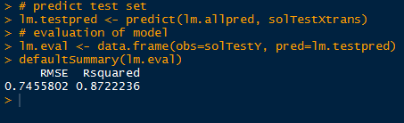Predict and Evaluate

With the predicted solubility values in lm.testpred, we evaluate the fit of the model with the true solubility test data in solTestY. We arrive at the evaluation by putting the two variables into a data.frame and calling the defaultSummary() function, available from the caret package. This displays the mean squared error and the R2.

Recall that the residual standard error with the training data was 0.5524, and now with the test set, we can say that the residual standard error, expected higher, was 0.7456. Also the R2 was lower in the test data set at 0.8722 compared to the training 0.9446.

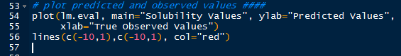Plotting Predicted and True Values

We can also plot the predicted solubility values against the true solubility values using plot(). Adding a y=x line using lines() gives us perspective to see how closely the predicted values align with the true values. Observe below, how most of the values, except for a few which are farther off, fall closely to the line- indicating similarity to the true values.

And there we have it, folks! In this post we used chemical descriptors to analyze and predict which compounds (QSAR modeling) are more likely to have different solubility levels, and which predictors (NumNonHAtoms, MolWeight, NumOxygen, and NumNonHBonds just for a few) are more significant in predicting compound solubility. It makes sense that  chemical descriptors indicating more complex chemical compound composition predict a chemical property, such as solubility.

This is just a sample of how new compounds are analyzed for specific properties computationally before more the expensive assays. Stay tuned for more regression analysis- such as robust regression and partial least squares!

Thanks for reading,


Wayne
@beyondvalence