KDD Cup: Profit Optimization in R Part 2: Decision Trees

Hello Readers,

This post continues the Knowledge Discovery and Data mining Cup case study from Part 1, where we explored the distribution and relationships of the target and predictor variables. Here in Part 2, we will build the decision trees to predict the target donation variable with predictor variables using the party R library. 

Recall that we are using decision trees to maximize returns (donations) from mail-in orders from many variables, including demographics, previous giving history, promotion history, and recency-frequency-donation variables. The data were used for the KDD 1998 Cup Competition.

cup98 Data

From Part 1 we created an abbreviated dataset consisting of 67 of the original 481 variables. Here we will subset more of the 67 variables down to 30 variables, including the target variable. The target variable is re-positioned as the first variable.

Training Set Code:

1 2 3 4 5 6 7 8 9 10 11 12 13 14 15 16 17 18 19 20 21 22 23 24 25 26 27 28 29 30 31 32 33 34 35 36 37 38 39 40 41 42

## 2. Training Decision Trees #### > library(party) # recursive 'PARTY'tioning # create new set > varSet2 <- c("AGE", "AVGGIFT", "CARDGIFT", "CARDPM12", + "CARDPROM", "CLUSTER2", "DOMAIN", "GENDER", "GEOCODE2", "HIT", + "HOMEOWNR", "HPHONE_D", "INCOME", "LASTGIFT", "MAXRAMNT", + "MDMAUD_F", "MDMAUD_R", "MINRAMNT", "NGIFTALL", "NUMPRM12", + "PCOWNERS", "PEPSTRFL", "PETS", "RAMNTALL", "RECINHSE", + "RFA_2A", "RFA_2F", "STATE", "TIMELAG") > cup98 <- cup98[, c("TARGET_D", varSet2)] > str(cup98) 'data.frame': 95412 obs. of 30 variables: $ TARGET_D: num 0 0 0 0 0 0 0 0 0 0 ... $ AGE : int 60 46 NA 70 78 NA 38 NA NA 65 ... $ AVGGIFT : num 7.74 15.67 7.48 6.81 6.86 ... $ CARDGIFT: int 14 1 14 7 8 3 8 4 8 1 ... $ CARDPM12: int 6 6 6 6 10 6 4 6 6 4 ... $ CARDPROM: int 27 12 26 27 43 15 26 14 29 11 ... $ CLUSTER2: int 39 1 60 41 26 16 53 38 57 34 ... $ DOMAIN : Factor w/ 17 levels " ","C1","C2",..: 12 8 6 6 9 12 12 12 6 11 ... $ GENDER : Factor w/ 7 levels " ","A","C","F",..: 4 6 6 4 4 1 4 4 6 6 ... $ GEOCODE2: Factor w/ 6 levels ""," ","A","B",..: 5 3 5 5 3 5 6 5 6 4 ... $ HIT : int 0 16 2 2 60 0 0 1 0 0 ... $ HOMEOWNR: Factor w/ 3 levels " ","H","U": 1 2 3 3 2 1 2 3 3 1 ... $ HPHONE_D: int 0 0 1 1 1 0 1 1 1 0 ... $ INCOME : int NA 6 3 1 3 NA 4 2 3 NA ... $ LASTGIFT: num 10 25 5 10 15 15 11 11 22 15 ... $ MAXRAMNT: num 12 25 16 11 15 16 12 11 22 15 ... $ MDMAUD_F: Factor w/ 4 levels "1","2","5","X": 4 4 4 4 4 4 4 4 4 4 ... $ MDMAUD_R: Factor w/ 5 levels "C","D","I","L",..: 5 5 5 5 5 5 5 5 5 5 ... $ MINRAMNT: num 5 10 2 2 3 10 3 5 10 3 ... $ NGIFTALL: int 31 3 27 16 37 4 14 5 11 3 ... $ NUMPRM12: int 14 13 14 14 25 12 9 12 12 9 ... $ PCOWNERS: Factor w/ 2 levels " ","Y": 1 1 1 1 1 1 2 1 1 1 ... $ PEPSTRFL: Factor w/ 2 levels " ","X": 2 1 2 2 1 2 2 1 2 1 ... $ PETS : Factor w/ 2 levels " ","Y": 1 1 1 1 1 1 2 1 1 1 ... $ RAMNTALL: num 240 47 202 109 254 51 107 31 199 28 ... $ RECINHSE: Factor w/ 2 levels " ","X": 1 1 1 1 2 1 1 1 1 1 ... $ RFA_2A : Factor w/ 4 levels "D","E","F","G": 2 4 2 2 3 3 2 2 3 3 ... $ RFA_2F : int 4 2 4 4 2 1 1 3 1 1 ... $ STATE : Factor w/ 57 levels "AA","AE","AK",..: 20 9 33 9 14 4 21 24 18 48 ... $ TIMELAG : int 4 18 12 9 14 6 4 6 8 7 ...

Setting Parameters

Before we train the decision trees, we need to set the parameters of the trees. The party library allows us to create trees with recursive binary 'party'tioning. First we determine the test (0.3) and training set (0.7) sizes to be created from the learning data. Then we set the "MinSplit" variable to 1000, the "MinBucket" to 400, the "MaxSurrogate" to 4, and the "MaxDepth" to 10. "MinSplit" is the minimum sum of weights in a node to be eligible to splitting; "MinBucket" is the minimum sum of weights in a terminal node; "MaxSurrogate" is the number of surrogate splits to evaluate; "MaxDepth" is the maximum depth of the tree. Surrogate splits are evaluated from other predictors after the best predictor is determined for splitting, and they are stored with each primary split.

Parameter Code:

1 2 3 4 5 6 7 8 9 10 11 12 13 14 15 16

# set parameters > nRec <- dim(cup98)[1] > trainSize <- round(nRec*0.7) > testSize <- nRec - trainSize ## ctree parameters > MinSplit <- 1000 > MinBucket <- 400 > MaxSurrogate <- 4 > MaxDepth <- 10 # can change > (strParameters <- paste(MinSplit, MinBucket, MaxSurrogate, + MaxDepth, sep="-")) [1] "1000-400-4-10" # number of loops > LoopNum <- 9 ## cost for each contact is $0.68 > cost <- 0.68

Observe the string "strParameters" to capture the decision tree parameters. We also store the number of decision trees to generate in "LoopNum" as 9, and the cost of each mail-in order as 0.68 cents in "cost".

Looping Decision Trees

Why do you want to create a "strParameters" variable? This will become evident soon, and it involves being able to run additional decision trees under different parameters to test the predicted donation values.

Because we are creating multiple decision trees (LoopNum=9), I advocate using a for loop to iterate through each tree, saving and writing the data for each. In each iteration we shall incorporate the decision tree plot, as well as the plotted cumulative donation amount sorted in decreasing order. 

The output will be written in a pdf file, using the pdf() function to start the R graphics device, and delineated by printing the "strParameters" and "LoopNumber" to track the loop output. At the end of each loop there will be 10 trees, with 9 being iterated and the 10th being the average of the 9. We take the average of the 9 trees in an attempt to eliminate partitioning errors. Since in a single tree the partitioning can distort the results of the test and training data, using 9 runs will incorporate different partitioning patterns.

So the first step is to open the pdf() graphics device, and set the out document name including the "strParameters". Then in the output we print out the parameters, and create the three result matrices for total donation, average donation, and donation percentile.

For Loop Decision Tree Code:

1 2 3 4 5 6 7 8 9 10 11 12 13 14 15 16 17 18 19 20 21 22 23 24 25 26 27 28 29 30 31 32 33 34 35 36 37 38 39 40 41 42 43 44 45 46 47 48 49 50 51 52 53 54 55 56 57 58 59 60 61 62 63 64

## run 9 times for tree building and use avg result > pdf(paste("evaluation-tree-", strParameters, ".pdf", sep=""), + width=12, height=9, paper="a4r", pointsize=6) > cat(date(), "\n") > cat(" trainSize=", trainSize, ", testSize=", testSize, "\n") > cat(" MinSplit=", MinSplit, ", MinBucket=", MinBucket, + ", MaxSurrogate=", MaxSurrogate, ", MaxDepth=", MaxDepth, + "\n\n") # run for multiple times and get the average result > allTotalDonation <- matrix(0, nrow=testSize, ncol=LoopNum) > allAvgDonation <- matrix(0, nrow=testSize, ncol=LoopNum) > allDonationPercentile <- matrix (0, nrow=testSize, ncol=LoopNum) > for (loopCnt in 1:LoopNum) { > cat(date(), ": iteration = ", loopCnt, "\n") # split into training data and testing data > trainIdx <- sample(1:nRec, trainSize) > trainData <- cup98[trainIdx,] > testData <- cup98[-trainIdx,] # train a decision tree > cup.Ctree <- ctree(TARGET_D ~ ., data=trainData, + controls=ctree_control(minsplit=MinSplit, + minbucket=MinBucket, + maxsurrogate=MaxSurrogate, + maxdepth=MaxDepth)) # size of tree > print(object.size(cup.Ctree), units="auto") > save(cup.Ctree, file=paste("cup98-ctree-", strParameters, + "-run-", loopCnt, ".rdata", sep="")) > figTitle <- paste("Tree", loopCnt) > plot(cup.Ctree, main=figTitle, type="simple", + ip_args=list(pval=FALSE), ep_args=list(digits=0, abbreviate=TRUE), + tp_args=list(digits=2)) # print(cup.Ctree) # test > pred <- predict(cup.Ctree, newdata=testData, type="response") > plot(pred, testData$TARGET_D) > print(sum(testData$TARGET_D[pred > cost] - cost)) # build donation matrices # quicksort used to random tie values > s1 <- sort(pred, decreasing=TRUE, method="quick", + index.return=TRUE) > totalDonation <- cumsum(testData$TARGET_D[s1$ix]) # cumulative sum > avgDonation <- totalDonation / (1:testSize) > donationPercentile <- 100 * totalDonation / sum(testData$Target_D) > allTotalDonation[,loopCnt] <- totalDonation > allAvgDonation[,loopCnt] <- avgDonation > allDonationPercentile[,loopCnt] <- donationPercentile > plot(totalDonation, type="l") > grid() } > graphics.off() > cat(date(), ": Loop Completed. \n\n\n") > fnlTotalDonation <- rowMeans(allTotalDonation) > fnlAveDonation <- rowMeans(allAvgDonation) > fnlDonationPercentile <- rowMeans(allDonationPercentile)

After we sample the index to create the training and test data, we run the tree using ctree(), and save the binary-tree object to its "strParameters" and current loop number designation as a RDATA file. In the pdf file, we print the tree structure, a scatter plot of the predicted and test data donations, and a cumulative test donation plot ordered by predicted donation size. The last plot examines how the decision tree models large donations, with a high initial increase indicating a good fit. The three result matrices are filled by column as each loop is completed.

Console Output

Depending on your computer, the loop might take a moments to a few minutes. The output begins with printing the date and time and parameters of the decision tree loop initialization. Once the loop begins, it starts to print the time at the start of each loop with the loop counter number. Then prints the size of the binary-tree object size, and in a new line, the predicted total donation profit, not including predicted donations less than the cost ($0.68). That segment repeats 9 times (the loop number), and prints the finished date and time in the end message.

Console Output Code:

1 2 3 4 5 6 7 8 9 10 11 12 13 14 15 16 17 18 19 20 21 22 23 24 25 26 27 28 29 30 31 32 33 34 35 36 37 38 39 40 41 42 43 44 45 46 47 48 49

> cat(date(), "\n") Wed May 28 09:30:53 2014 > cat(" trainSize=", trainSize, ", testSize=", testSize, "\n") trainSize= 66788 , testSize= 28624 > cat(" MinSplit=", MinSplit, ", MinBucket=", MinBucket, + ", MaxSurrogate=", MaxSurrogate, ", MaxDepth=", MaxDepth, + "\n\n") MinSplit= 1000 , MinBucket= 400 , MaxSurrogate= 4 , MaxDepth= 10 Wed May 28 09:32:18 2014 : iteration = 1 25.6 Mb [1] 3772.87 Wed May 28 09:33:27 2014 : iteration = 2 6.5 Mb [1] 4297.76 Wed May 28 09:34:20 2014 : iteration = 3 29.2 Mb [1] 3483.43 Wed May 28 09:35:23 2014 : iteration = 4 31.8 Mb [1] 4056.56 Wed May 28 09:36:26 2014 : iteration = 5 24.6 Mb [1] 4258.46 Wed May 28 09:37:27 2014 : iteration = 6 30.2 Mb [1] 2584.28 Wed May 28 09:38:29 2014 : iteration = 7 26.1 Mb [1] 3515.26 Wed May 28 09:39:32 2014 : iteration = 8 21.4 Mb [1] 3706.14 Wed May 28 09:40:32 2014 : iteration = 9 34.9 Mb [1] 4426.24 > graphics.off() > cat(date(), ": Loop Completed. \n\n\n") Wed May 28 09:41:44 2014 : Loop Completed. > fnlTotalDonation <- rowMeans(allTotalDonation) > fnlAveDonation <- rowMeans(allAvgDonation) > fnlDonationPercentile <- rowMeans(allDonationPercentile) > rm(trainData, testData, pred) > results <- data.frame(cbind(allTotalDonation, fnlTotalDonation)) > names(results) <- c(paste("run", 1:LoopNum), "Average") > write.csv(results, paste("evaluation-TotalDonation-", strParameters, + ".csv", sep="")) >

The last portion of the console output code covers the average donation values over all 9 trees. Out of the "fnlTotalDonation", "fnlAveDonation", and "fnlDonationPercentile", we save the "allTotalDonation" and the "fnlTotalDonation". These variables include the cumulative donations and the average cumulative donations, saved in a CSV file designated by "strParameters".

PDF Output

Let us examine the output the code wrote to the pdf file. For our current "strParameters" we find the pdf file named "evaluation-tree-1000-400-4-10.pdf". Opening the file, we discover 9 sets of plots: a binary-tree plot, a scatter plot of predicted and test donation values, and a plot of the cumulative test donations ordered by predicted donation size.

Below I display the first set of plots of the first tree. We begin with the decision tree:

Notice that it first splits at the variable, "LastGift". And next is the regression plot detailing test donations and predicted values:

We see the discrete predicted values on the x-axis versus the more continuous test donation values. There is not much noticeable correlation. And lastly the cumulative test donation plot, is indexed by decreasing predicted donations:

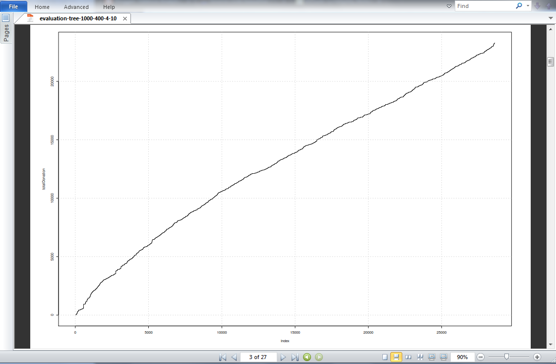
We have a steadily increasing cumulative donation plot, indicating that the tree model did an average job in predicting high donations. The actual donations were indexed by the highest predicted donations so actual high donations should have been plotted first on the x-axis, leading to a sharp increase in the y value at the beginning of the plot.

CSV Output

In our CSV output we saved the "allTotalDonation" and "fnlTotalDonation". The CSV file should be named "evaluation-TotalDonation-1000-400-4-10.csv". Using read.csv() to read in the file, we print out the first fifteen rows of the results. The first column is the index, followed by nine columns of "run.x" loop number, and the average cumulative donation for all nine runs.

CSV Output Code:

1 2 3 4 5 6 7 8 9 10 11 12 13 14 15 16 17 18 19 20 21 22 23 24 25 26 27

> ## 3. interpret results #### > results <- read.csv(paste("evaluation-TotalDonation-", strParameters, ".csv", sep="")) > results[1:15,] X run.1 run.2 run.3 run.4 run.5 run.6 run.7 run.8 run.9 Average 1 1 0 0 0 0 0 0 0 0 0 0.000000 2 2 0 0 10 0 0 0 0 0 0 1.111111 3 3 0 0 10 0 0 0 0 0 0 1.111111 4 4 0 0 10 0 0 0 0 0 0 1.111111 5 5 0 0 10 0 0 0 0 0 50 6.666667 6 6 0 0 10 0 0 0 0 0 50 6.666667 7 7 0 0 10 0 0 0 0 0 50 6.666667 8 8 0 0 10 0 0 0 0 0 50 6.666667 9 9 0 0 10 0 0 0 0 0 50 6.666667 10 10 0 13 10 0 0 0 0 0 50 8.111111 11 11 0 13 10 0 0 0 0 0 50 8.111111 12 12 0 13 10 0 0 0 0 0 50 8.111111 13 13 0 13 10 0 0 0 0 0 50 8.111111 14 14 0 13 10 0 0 0 0 0 50 8.111111 15 15 0 13 27 0 0 0 0 0 50 10.000000 > tail(results) X run.1 run.2 run.3 run.4 run.5 run.6 run.7 run.8 run.9 Average 28619 28619 23264.82 23762.08 22536.67 23885.04 23082.46 21699.42 22479 22477.25 23217.17 22933.77 28620 28620 23284.82 23762.08 22536.67 23885.04 23082.46 21699.42 22479 22477.25 23217.17 22935.99 28621 28621 23284.82 23762.08 22536.67 23885.04 23082.46 21699.42 22479 22477.25 23217.17 22935.99 28622 28622 23284.82 23762.08 22536.67 23885.04 23082.46 21699.42 22504 22477.25 23217.17 22938.77 28623 28623 23284.82 23762.08 22536.67 23885.04 23082.46 21699.42 22504 22477.25 23247.17 22942.10 28624 28624 23284.82 23762.08 22536.67 23885.04 23082.46 21699.42 22504 22477.25 23247.17 22942.10

Next we print out the last six rows with tail(), which displays the cumulative results of each run and the average cumulative donation (not including cost). The average total cumulative donation summed to $22,942.10. Among the runs, ranged from $21,699.42 for run six to $23,885.02 for run four.

Again, this is turning into a lengthy post. After running the loop for one "strParameters" set, we have the predicted donation data. Being optimization, later we will run different "strParameters" to determine which set of models can predict the highest donation return. The next post will explore the donation results data with graphs, in preparation for selecting the best set of decision trees. Stay tuned for more posts!


Thanks for reading,

Wayne
@beyondvalence
LinkedIn

More:
1. KDD Cup: Profit Optimization in R Part 1: Exploring Data
2. KDD Cup: Profit Optimization in R Part 2: Decision Trees
3. KDD Cup: Profit Optimization in R Part 3: Visualizing Results
4. KDD Cup: Profit Optimization in R Part 4: Selecting Trees
5. KDD Cup: Profit Optimization in R Part 5: Evaluation

KDD Cup: Profit Optimization in R Part 1: Exploring Data

Hello Readers,

Today we begin a case study on predicting and optimizing customer response and maximizing donations. The data were obtained from the Knowledge Discovery in Data (KDD) Cup's 1998 competition. KDD is a Special Interest Group of the Association of Computing Machinery (ACM). Here is a link to the annual KDD conference in 2014 titled "Data Mining for Social Good" in NYC.

KDD Logo

We will train decision trees to predict which customers donate the most, and optimize who to send the mail-in orders. Here we shall use the party library in R. The KDD data can be downloaded here. After you decompress the files, you will need cup98LRN.txt (training set) and cup98VAL.txt (test set).

Part 1

In this first post, we will explore the data, and visualize the distributions of the target variable and its relationship with other variables. In Part 2 I will cover building the decision trees, next in Part 3 I shall visualize the donation results, and in Part 4 I will finish by talking about selecting the best tree to maximize donations.

The 1998 KDD Data

First off, this is a large learning dataset with 95,412 rows and 481 variables at 117 MB uncompressed. Likewise, the test set is of similar dimension and size. Therefore we would have to explore the data and determine which variables we want to use to predict donations, and locate the donation amount variable. Note that there is a data dictionary detailing all the variables in the information section of the data tab.

To grasp what data we are dealing with, we use the describe() function from the Hmisc library. As you can see, along with mean, unique and missing values, median, and quantiles, it also displays the highest and lowest values. We pass the first 28 variables to describe(), which covers the demographic data. The output is quite lengthy, so if you want to run the other section of variables, you can uncomment them.

Describing Demographics Code:

1 2 3 4 5 6 7 8 9 10 11 12 13 14 15 16 17 18 19 20 21 22 23 24 25 26 27 28 29 30 31 32 33 34 35 36 37 38 39 40 41 42 43 44 45 46 47 48 49 50 51 52 53 54 55 56 57 58 59 60 61 62 63 64 65 66 67 68 69 70 71 72 73 74 75 76 77 78 79 80 81 82 83 84 85 86 87 88 89 90 91 92 93 94 95 96 97 98 99 100 101 102 103 104 105 106 107 108 109 110 111 112 113 114 115 116 117 118 119 120 121 122 123 124 125 126 127 128 129 130 131 132 133 134 135 136 137 138 139 140 141 142 143 144 145 146 147 148 149 150 151 152 153 154 155 156 157 158 159 160 161 162 163 164 165 166 167 168 169 170 171 172 173 174 175 176 177 178 179 180 181 182 183 184 185 186 187 188 189 190 191 192 193 194 195 196 197 198 199 200 201 202 203 204 205 206 207 208 209 210 211

# learning dataset # 95,412 records, 481 fields # 2 target variables # load learning data ### > cup98 <- read.csv("cup98LRN.txt", sep=",") ## 1. detailed description of the variables #### # target variables ## TARGET_B (y-n donation) and TARGET_D (donation amount) > library(Hmisc) # describe(cup98[,1:28]) # demographics # describe(cup98[,29:42]) # response to other types of mail orders # describe(cup98[,43:55]) # overlay data # describe(cup98[,56:74]) # donor interests # describe(cup98[,75]) # PEP star RFA status # describe(cup98[,76:361]) # characteristics of donor neighborhood # describe(cup98[,362:407]) # promotion history # describe(cup98[,408:412]) # summary variables of promotion history # describe(cup98[,413:456]) # giving history # describe(cup98[,457:469]) # summary variables of giving history # describe(cup98[,470:473]) ## ID & TARGETS # describe(cup98[,474:479]) # RFA (recency-frequency-donation amount) # describe(cup98[,480:481]) # cluster & geocode # names(cup98) > describe(cup98[,1:28]) # demographics cup98[, 1:28] 28 Variables 95412 Observations ----------------------------------------------------------------------------------------------- ODATEDW n missing unique Mean .05 .10 .25 .50 .75 .90 .95 95412 0 54 9141 8601 8601 8801 9201 9501 9601 9601 lowest : 8306 8401 8501 8601 8604, highest: 9510 9511 9512 9601 9701 ----------------------------------------------------------------------------------------------- OSOURCE n missing unique 95412 0 896 lowest : AAA AAD AAM ABC, highest: YAN YKA YKD YNF ZOY ----------------------------------------------------------------------------------------------- TCODE n missing unique Mean .05 .10 .25 .50 .75 .90 .95 95412 0 55 54.22 0 0 0 1 2 28 28 lowest : 0 1 2 3 4, highest: 24002 28028 39002 58002 72002 ----------------------------------------------------------------------------------------------- STATE n missing unique 95412 0 57 lowest : AA AE AK AL AP, highest: VT WA WI WV WY ----------------------------------------------------------------------------------------------- ZIP n missing unique 95412 0 19938 lowest : 00801 00802 00820 00821 00840 , highest: 99901- 99925 99928 99928- 99950 ----------------------------------------------------------------------------------------------- MAILCODE n missing unique 95412 0 2 (94013, 99%), B (1399, 1%) ----------------------------------------------------------------------------------------------- PVASTATE n missing unique 95412 0 3 (93954, 98%), E (5, 0%), P (1453, 2%) ----------------------------------------------------------------------------------------------- DOB n missing unique Mean .05 .10 .25 .50 .75 .90 .95 95412 0 947 2724 0 0 201 2610 4601 5605 6201 lowest : 0 1 2 4 5, highest: 9701 9704 9706 9708 9710 ----------------------------------------------------------------------------------------------- NOEXCH n missing unique 95412 0 4 (7, 0%), 0 (95085, 100%), 1 (285, 0%), X (35, 0%) ----------------------------------------------------------------------------------------------- RECINHSE n missing unique 95412 0 2 (88709, 93%), X (6703, 7%) ----------------------------------------------------------------------------------------------- RECP3 n missing unique 95412 0 2 (93395, 98%), X (2017, 2%) ----------------------------------------------------------------------------------------------- RECPGVG n missing unique 95412 0 2 (95298, 100%), X (114, 0%) ----------------------------------------------------------------------------------------------- RECSWEEP n missing unique 95412 0 2 (93795, 98%), X (1617, 2%) ----------------------------------------------------------------------------------------------- MDMAUD n missing unique 95412 0 28 lowest : C1CM C1LM C1MM C2CM C2LM, highest: L1MM L2CM L2LM L2TM XXXX ----------------------------------------------------------------------------------------------- DOMAIN n missing unique 95412 0 17 C1 C2 C3 R1 R2 R3 S1 S2 S3 T1 T2 T3 U1 U2 U3 Frequency 2316 6145 8264 5280 1358 13623 4809 11503 8530 1891 4982 12369 2176 4510 3254 2598 % 2 6 9 6 1 14 5 12 9 2 5 13 2 5 3 3 U4 Frequency 1804 % 2 ----------------------------------------------------------------------------------------------- CLUSTER n missing unique Mean .05 .10 .25 .50 .75 .90 .95 93096 2316 53 27.92 4 8 15 28 40 47 50 lowest : 1 2 3 4 5, highest: 49 50 51 52 53 ----------------------------------------------------------------------------------------------- AGE n missing unique Mean .05 .10 .25 .50 .75 .90 .95 71747 23665 96 61.61 34.3 39.0 48.0 62.0 75.0 83.0 87.0 lowest : 1 2 3 4 6, highest: 94 95 96 97 98 ----------------------------------------------------------------------------------------------- AGEFLAG n missing unique 95412 0 3 (29548, 31%), E (57344, 60%), I (8520, 9%) ----------------------------------------------------------------------------------------------- HOMEOWNR n missing unique 95412 0 3 (22228, 23%), H (52354, 55%), U (20830, 22%) ----------------------------------------------------------------------------------------------- CHILD03 n missing unique 95412 0 4 (94266, 99%), B (40, 0%), F (237, 0%), M (869, 1%) ----------------------------------------------------------------------------------------------- CHILD07 n missing unique 95412 0 4 (93846, 98%), B (97, 0%), F (408, 0%), M (1061, 1%) ----------------------------------------------------------------------------------------------- CHILD12 n missing unique 95412 0 4 (93601, 98%), B (142, 0%), F (520, 1%), M (1149, 1%) ----------------------------------------------------------------------------------------------- CHILD18 n missing unique 95412 0 4 (92565, 97%), B (263, 0%), F (1142, 1%), M (1442, 2%) ----------------------------------------------------------------------------------------------- NUMCHLD n missing unique Mean 12386 83026 7 1.528 1 2 3 4 5 6 7 Frequency 7792 3110 1101 316 59 7 1 % 63 25 9 3 0 0 0 ----------------------------------------------------------------------------------------------- INCOME n missing unique Mean 74126 21286 7 3.886 1 2 3 4 5 6 7 Frequency 9022 13114 8558 12732 15451 7778 7471 % 12 18 12 17 21 10 10 ----------------------------------------------------------------------------------------------- GENDER n missing unique 95412 0 7 A C F J M U Frequency 2957 2 2 51277 365 39094 1715 % 3 0 0 54 0 41 2 ----------------------------------------------------------------------------------------------- WEALTH1 n missing unique Mean .05 .10 .25 .50 .75 .90 .95 50680 44732 10 5.346 1 1 3 6 8 9 9 0 1 2 3 4 5 6 7 8 9 Frequency 2413 3454 4085 4237 4810 5280 5825 6198 6793 7585 % 5 7 8 8 9 10 11 12 13 15 ----------------------------------------------------------------------------------------------- HIT n missing unique Mean .05 .10 .25 .50 .75 .90 .95 95412 0 75 3.321 0 0 0 0 3 11 17 lowest : 0 1 2 3 4, highest: 75 79 84 240 241 -----------------------------------------------------------------------------------------------

Our focus on the targets lead us to variables 470 to 473. They include the CONTROLN as the unique id number, TARGET_B as a binary donation indicator, TARGET_D as the donation amount in USD, HPHONE_D as a binary home phone number indicator.

Target: Donations

Let us take a look at the distribution of the donation variable, TARGET_D. From the describe() function we see the majority of the donations are small denominations, with 95% being 3 dollars or less. However, in the extreme values, we see 100+ dollar donations, peaking at $200.

Describing Donations Code:

1 2 3 4 5 6 7 8 9

> describe(cup98[,472]) cup98[, 472] n missing unique Mean .05 .10 .25 .50 .75 95412 0 71 0.7931 0 0 0 0 0 .90 .95 0 3 lowest : 0.0 1.0 2.0 2.5 3.0 highest: 100.0 101.0 102.0 150.0 200.0

We can isolate the positive donations in cup98pos by using TARGET_B > 0, and visualize the modified donation distribution using a box plot. This way we only deal with those rows that donated some amount.

Plotting Donations Code:

1 2 3 4 5 6 7

> # positive donations- boxplot, description #### > cup98pos <- cup98[cup98$TARGET_B > 0,] > donations <- cup98pos$TARGET_D > summary(donations) Min. 1st Qu. Median Mean 3rd Qu. Max. 1.00 10.00 13.00 15.62 20.00 200.00 > boxplot(donations, main="Positive Donations")

A large portion- between 25th and 75th percentiles- 50% of the values lie at or below 20 dollars. So we can conclude among those who donated, they usually donated $20 or less. However there were a few generous donations of $100-$200. The boxplot offers a fast way to view distributions. Another option is to cut() the donations into intervals and see how many rows fall into each interval. 

We split the interval into multiples of 5, with the lowest from 0 to 0.1, and the highest covering 50-200. Observing the table of the donation intervals, we see the majority (n=90569) did not donate anything, while 110 donations fell into the highest category, 50-200 dollars. We plot both the donation intervals and the positive donation intervals to examine the distribution more closely.

Cut and Plot Code:

1 2 3 4 5 6 7 8 9 10 11 12 13 14 15 16

# create level factor donation variable #### # [a,b), closed on left, open on right: (a <= x < b) > cup98$TARGET_D2 <- cut(cup98$TARGET_D, right=FALSE, breaks=c(0,0.1,10,15,20,25,30,50,max(cup98$TARGET_D))) > cup98pos$TARGET_D2 <- cut(cup98pos$TARGET_D, right=FALSE, breaks=c(0,0.1,10,15,20,25,30,50,max(cup98pos$TARGET_D))) > layout(matrix(c(1,2),2,1)) > plot(table(cup98$TARGET_D2), main="All Donations", xlab="Dollar Amount", ylab="Numer of Donations") > plot(table(cup98pos$TARGET_D2), main="Positive Donations", xlab="Dollar Amount", ylab="Numer of Donations") > layout(1) > table(cup98$TARGET_D2) [0,0.1) [0.1,10) [10,15) [15,20) [20,25) [25,30) [30,50) [50,200) 90569 1132 1378 806 745 435 233 110

In the lower plot you notice the difference in only with those who donated due to the small y-axis limit so you can see the bars more clearly in the lower scale. The most frequent donation intervals include [0.1,10) and [10,15). Remember that [ ] are closed which include the number and ( ) are open, which do not include the number. So the interval [10,15) describes the interval 10 and up to, but not including 15.

Additionally, we can plot the discrete values piped from the table() function, which outputs a named vector of the number of donations for each unique donation value. This way we can visualize the number of donations for each dollar amount, instead of relying on intervals, as we did above.

Plot Code:

1 2 3 4

# discrete donation plot > plot(table(cup98pos$TARGET_D), type="l", ylim=c(0,1000), + xlab="Donation Amount", ylab="Number of Donations", + main="Donation Distribution")

The tick marks on the x-axis denote actual donated amounts, and the y-axis show the number of donations at that donation amount. Observe the majority of the donations are below $27, while the highest 4 peaks are above 400- the 5th comes in close at 392, which is the $25 amount. The distribution is heavily skewed to the right, with the majority of the values less than the large extreme to the right.

Variable Selection

Because there are a large number of variables from which to select, going through each might be a hassle. Luckily, we have a data dictionary describing each variable. We will select 67 of the 481 variables available from the cup98 data. They include demographic variables, donor interests, promotion history, giving history, ID & TARGETs, and recency-frequency-donation amounts. Of course you can add other variables you think will be vital in predicting donation amounts. 

Variable Selection Code:

1 2 3 4 5 6 7 8 9 10 11 12 13 14 15 16 17 18 19 20 21 22 23 24 25 26 27

> # select variables #### > varSet <- c( + # demographics 160 R and Data Mining + "ODATEDW", "OSOURCE", "STATE", "ZIP", "PVASTATE", "DOB", + "RECINHSE", "MDMAUD", "DOMAIN", "CLUSTER", "AGE", "HOMEOWNR", + "CHILD03", "CHILD07", "CHILD12", "CHILD18", "NUMCHLD", + "INCOME", "GENDER", "WEALTH1", "HIT", + # donor interests + "COLLECT1", "VETERANS", "BIBLE", "CATLG", "HOMEE", "PETS", + "CDPLAY", "STEREO", "PCOWNERS", "PHOTO", "CRAFTS", "FISHER", + "GARDENIN", "BOATS", "WALKER", "KIDSTUFF", "CARDS", "PLATES", + # PEP star RFA status + "PEPSTRFL", + # summary variables of promotion history + "CARDPROM", "MAXADATE", "NUMPROM", "CARDPM12", "NUMPRM12", + # summary variables of giving history + "RAMNTALL", "NGIFTALL", "CARDGIFT", "MINRAMNT", "MAXRAMNT", + "LASTGIFT", "LASTDATE", "FISTDATE", "TIMELAG", "AVGGIFT", + # ID & targets + "CONTROLN", "TARGET_B", "TARGET_D", "TARGET_D2", "HPHONE_D", + # RFA (Recency/Frequency/Donation Amount) + "RFA_2F", "RFA_2A", "MDMAUD_R", "MDMAUD_F", "MDMAUD_A", + #others + "CLUSTER2", "GEOCODE2") > > # created new cup98 set #### > cup98 <- cup98[, varSet]

Since we have created the new cup98 dataset, we are now ready to create the decision trees. But before we move on, let us explore some of the predictor variables included in the new cup98 data.

Variable Distribution

First, let us start with exploring age and donation amount. We will create a new positive donation dataset from the new cup98 data, and cut() the AGE variable into increments of 5. Then we will plot the donation stratified by the new age intervals to examine how each age grouping donated. Note that we restrict the donation plotted on the y-axis to a maximum of $40.

Donation Age Distribution Code:

1 2 3 4 5 6 7

# check distribution of donation in various age groups #### > cup98pos <- cup98[cup98$TARGET_D>0,] > age2 <- cut(cup98pos$AGE, right=FALSE, breaks=seq(0, 100, by=5)) table(age2) > boxplot(cup98pos$TARGET_D ~ age2, ylim=c(0,40), las=3, + main="Donation Age Distribution") # people aged 30..60 have higher median donation; in workforce

Examining the boxplots above, we see that the plots with intervals from 30 to 60 have the highest median donation amount. For practical purposes, the age of donation begins in the 15 to 20 age group, and continues all the way to the 95 to 100 group. A major reason why people aged 30 to 60 donate the higher amounts, can be attributed to their workforce status. People at those ages are most likely to have a job, and therefore has the disposable income to donate.

Next, we can look at the gender of donor with positive donations. We will focus on female, male and joint account donors. This time, with less categories, we can use a density plot to overlay the female, male, and joint plots. Note that we attach() the cup98pos to add it to the R's search path, so we do not have to type the name over and over. Again we restrict the donation amount to the lower donation band, but this time from 0 to 60 to capture the majority of the donations.

Donation-Gender Distribution Code:

1 2 3 4 5 6 7 8 9 10 11 12

# check distribution of donation for gender #### > attach(cup98pos) ## density plot for male-female-Joint donations > plot(density(TARGET_D[GENDER=="F"]), xlim=c(0,60), col=1, lty=1, main="Donation Density Plot for Gender") > lines(density(TARGET_D[GENDER=="M"]), col=2, lty=2) > lines(density(TARGET_D[GENDER=="J"]), col=3, lty=3) > legend("topright", c("Female", "Male", "Joint account"), col=1:3, lty=1:3) > detach(cup98pos)

Observe the 3 different colored and patterned lines for the female, male, and joint account densities. All three categories have the similar peak at 10 dollars, and both female and male have similar peaks. However, joint account donations do not have peaks at 5, 15, 20, or 25 amounts. Can you guess that the donation amounts are mainly in multiples of 5 (for donation options in the mail-in order)?

Variable Correlations

We can also check the correlations between the target donation variable and other numeric variables. First create an index indicating whether it is numeric or not. Then we correlate the target donation variable with those in cup98 using the numeric index. We make it easier by taking the absolute value of the correlation, and ordering them in decreasing order with the highest correlation first. This way we will observe the variables with the strongest correlation in the beginning.

Correlation Code:

1 2 3 4 5 6 7 8 9 10 11 12 13 14 15 16 17 18

# check correlation between target & numeric vars #### > num.idx <- which(sapply(cup98, is.numeric)) > correlations <- cor(cup98$TARGET_D, cup98[,num.idx], + use="pairwise.complete.obs") > correlations <- abs(correlations) > (correlations <- correlations[,order(correlations, decreasing=TRUE)]) TARGET_D TARGET_B LASTGIFT RAMNTALL AVGGIFT 1.0000000000 0.7742323755 0.0616784458 0.0448101061 0.0442990841 MAXRAMNT INCOME CLUSTER2 NUMPRM12 WEALTH1 0.0392237509 0.0320627023 0.0290870830 0.0251337775 0.0248673117 MINRAMNT LASTDATE NUMPROM CLUSTER CARDPM12 0.0201578686 0.0188471021 0.0173371740 0.0171274879 0.0163577542 NUMCHLD CONTROLN CARDPROM FISTDATE ODATEDW 0.0149204899 0.0133664439 0.0113023931 0.0075324932 0.0069484311 HIT CARDGIFT NGIFTALL MAXADATE TIMELAG 0.0066483728 0.0064498822 0.0048990126 0.0044963520 0.0036115917 DOB HPHONE_D AGE RFA_2F 0.0027541472 0.0024315898 0.0022823598 0.0009047682

Of course TARGET_D correlates perfectly with itself, and TARGET_B correlates highly as well, being a yes/no indicator of donation. The next variables with higher correlations are LASTGIFT, RAMNTALL, and AVGGIFT, all three measures of previous giving history. This indicates (with common sense) that previous history is likely to be a strong predictor of the current donation amount.

We can create a scatter plot of the variable HIT, which measures the number of mail-order responses and age. This gives us an idea on how many responses were received from each age. We further stratify the plot by donation amount, changing the shape and color depending on a non-zero donation or not.

Plotting Donation Responses Code:

1 2 3 4 5 6 7 8 9

## scatter plot for donation response and age > color <- ifelse(cup98$TARGET_D > 0, "blue", "black") > pch <- ifelse(cup98$TARGET_D > 0, "+", ".") > plot(jitter(cup98$AGE), jitter(cup98$HIT), pch=pch, col=color, cex=0.7, ylim=c(0,70), xlab="AGE", ylab="HIT", main="Mail Order Responses By Age and Donation Status") > legend("topleft", c("TARGET_D>0", "TARGET_D=0"), col=c("blue", "black"), pch=c("+", "."))

As we inspect the above plot, we notice the most mail-order responses come from older people, ages 60-80. However, those who donated did so in less responses. Though people would respond to the mail-in order, many which were sent back did not include a donation. There were donations in the responses from people who sent back less responses. It appears as if people want to donate, they would donate in the first few responses.

This post is getting lengthy already, so I will stop going through variables here, and continue the next post with building the decision trees to predict donations. Stay tuned for Part 2 of this Profit Optimization Case Study!


Thanks for reading,

Wayne
@beyondvalence
LinkedIn

More:
1. KDD Cup: Profit Optimization in R Part 1: Exploring Data
2. KDD Cup: Profit Optimization in R Part 2: Decision Trees
3. KDD Cup: Profit Optimization in R Part 3: Visualizing Results
4. KDD Cup: Profit Optimization in R Part 4: Selecting Trees
5. KDD Cup: Profit Optimization in R Part 5: Evaluation