R: Partial Least Squares Regression, RMSEP, and Components

Hello Readers,

Here we will continue our R regression series and after working with ordinary, and robust regression, we will address partial least squares regression. Using the same chemical descriptors data set, we will predict solubility of compounds with a different approach of looking at the predictors themselves and how they relate to each other. 

In many data sets, the predictors we use could be correlated to the response (what we are looking for) and to each other (not good for variability). If too many predictor variables are correlated to each other, then the variability would render the regression unstable.

One way to correct for predictor correlation is to use PCA or principle component analysis which seeks to find a linear combination of predictors to capture the most variance. The jth principal component (PC) can be written as:

PCj = (aj1 * predictor 1) + (aj2 * predictor 2) + ... + (ajp * predictor p)

However this method does not always produce a PC that correlates with the response variable as shown below:

From Max Kuhn's Applied Predictive Modeling

Whereas using partial least squares regression, we see that it is correlated with the response variable.

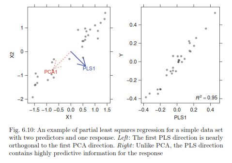
From Max Kuhn's Applied Predictive Modeling

So start R and let us look at partial least squares regression!

Partial Least Squares

PLS regression, like PCA, seeks to find components which maximize the variability of predictors but differs from PCA as PLS requires the components to have maximum correlation with the response. PLS is a supervised procedure whereas PCA is unsupervised.

First we require the following R packages, specifically the pls library:

R Packages

The Solubility data from the AppliedPredictiveModeling package is summarized and transformed in the ordinary regression post.

In the pls library, we will use the plsr() function for partial least squares regression. We specify the response variable as solubility, use all the predictor variables with a ".", and include cross-validation parameter as "CV".

plsr() and Prediction

With the familiar predict() function, use the plsFit list object which contains the predicted values for each component iteration of the PLSR algorithm, with default set at the Dayal and MacGregor kernel algorithm "kernelpls". We predict the first 5 solubility values "solTestXtrans[1:5, ]" using 1 and 2 components "ncomp=1:2". The results are shown below.

Solubility Values for 1 and 2 Components

But how do we know from what number of predictors to choose? Well there are several methods, let us take a look at the summary() output of plsFit, truncated into two parts. We look for component number which adequately explains both predictors and response variances.

The first section displays the root mean squared error of prediction (RMSEP), cross-validation estimate, as well as the adj-CV, which is adjusted for bias. Take note of the dimensions of X and Y of the data towards the top of the output.

pls Summary Part 1

The next section shows the percent of variance explained by components for predictors and response. See how the variance explained rises quickly from 1 component and stabilizes above 10..13 components. That would be a good component range for the pls model.

pls Summary Part 2

Another method is by plotting and locating the lowest Root Mean Standard Error of Prediction (RMSEP).

PLS Prediction Error

There are two methods able to produce the visualization of RMSEP. The first uses the function validationplot() from the pls package which will give us the RMSEP plot for each component iteration in the model. Specify the validation type to be "val.type=RMSEP".

validationplot()

We see from the validation plotting function that there is a sharp decrease in the root mean standard error for the first few numbers of components and then plateaus after about 10. Keep in mind the summary information about the explained variance increments stabilizing around 10.


However we want to find the component number corresponding to lowest point in the RMSEP. Using the RMSEP() function with estimate parameter set to "CV" we can derive the desired value. The plot() will give us the initial graph- see how similar it is to the plot obtained from validationplot(). (They should be the same.)

RMSEP() and plot()

To calculate the lowest RMSEP, we use the which.min() function, which returns the index of the lowest value. The minimum value is found at 10 components and we add a point to the plot using the points() function such that the x and y values are: (component number, minimum RMSEP value).

Finding Lowest RMSEP

The plot with the added locating point in red is shown below.

RMSEP() with points()

Using the training data, we can plot the predicted solubilities from the training set to the actual solubilities, using another plot() function:

plot(plsFit, ncomp=10, asp=1, line=True)

Checking Training Predictions

From the above plot, we see that the points mainly lie along the line. This is expected because the data is from the same training set used to create the plsr model.

Predicted Solubilities

Now that we have an optimal component number (10), we can go ahead and use the plsr model to predict new solubility values for test predictor data. Again we use the predict() function and specify the test data (solTestXtrans) and the number of components (ncomp=10).

Predicting Solubility from Test Data

Then we plot the observed ('test' data with actual values,  lucky us) and the predicted values together with a line, determining how close the values are.

And the plot does not look too bad, with no indication of anomalies.

Evaluation of plsr Model

Because we have the observed solubility values for the 'test' data we can evaluate how well the model performed. However in the usual circumstances, we would not know the actual values, hence what we are doing- predicting values from the test predictor data.

Using the observed values in solTestY and the predicted values in pls.pred2[,1,1], we can use the defaultSummary() function to obtain the RMSE and Rsquared, as shown below.

Evaluation

From the output, we see that the RMSE is around 0.7366, and the Rsquared is approximately 0.8744, explaining 87% of the test data variance.


And there we have it, folks! This (lengthy) post covered partial least squares regression in R, starting with fitting a model and interpreting the summary to plotting the RMSEP and finding the number of components to use. Then we predicted solubilities from the the test data with the plsr model we fitted to the training data.

Check back for more posts on predictive modeling! Happy programming guys!


Thanks for reading,

Wayne
@beyondvalence

R: Robust Regression and Estimation of Model Performance

Hello Readers,


Today we continue our discussion about regression in QSAR modeling and venture into robust regression and estimating the performance of the model using cross-validation. Using the chemical solubility data set from the QSAR post, we will explore more regression topics!


Let us start R and begin!

Robust Regression

In the previous regression post we talked about ordinary regression with multiple (chemical descriptor) predictors trying to model compound solubility. Again, we require the following R packages: MASS, caret, AppliedPredictiveModeling, lars, pls, and elasticnet.

R Packages

While using the Box-Cox transformed continuous variables in solTrainXtrans data set, we can perform robust regression with the rlm() function from MASS, similar to the lm() regression function in the last post. By default, the rlm() function uses the Huber approach to account for values which excessively influence the model by taking the sum of the differences instead of the sum of squared differences (SSE) above a threshold.

Robust Regression

Because there are so many predictors, the results are truncated to show the beginning and the end, where all types of predictors are shown.

End of Robust Regression

As we can see from the results above, the residual standard error was 0.3739. Previously, from the ordinary regression model, our RMSE was 0.5524, with the test prediction RMSE of 0.7456. Clearly we can see the difference from the two regression models, with the robust RMSE lower than the RMSE of the ordinary regression. Why? Because robust regression took into account larger residuals above a threshold and took the simple residual (difference), while using the squared residuals for smaller residuals. That is why we a smaller RMSE for the robust regression- it is more resistance to influential outliers.

Plotting the Predicted Values

We can visualize the robust regression results by using a plot of the predicted and true solubility values using predict() and plot().

Predicting rlm and Plotting Predicted Solubilities

Using the graph, we can compare the predicted values of the robust regression with those from the ordinary regression from the previous post by adding them as points() and creating a legend() to differentiate the two.

Adding Predicted Regression Solubilities and Legend

Which will yield us the graphic below:

As we can see, the two are very similar in distribution, while some predicted points between the two regression models vary.

Estimation of Model Performance

One method of evaluating how well the regression model fit an independent data set is through cross-validation, where we resample the entire data set in parts for the regression training. In other words, how well will the predictive model perform on an unknown data set? That is where cross-validation -a method of resampling- comes to our aid.

Using the trainControl() function, we can specify the type of resampling to be cross-validation with method="cv". Then with the train() function we input the predictor variables and response variable, and the resampling method is used as the type of control in trControl=ctrl.

Cross-Validation Regression

The subsequent summary is displayed below in three parts:

Cross-Validation Object

As we can see, the sample sizes (855, 855, 856, etc.) are roughly 90% of the samples because the data was split into 10 parts with 9 predicting the remain 1 which cycles through each of the 10 parts. Next we have the summary of coefficients.

Cross-Validation Summary Top

We obtain a residual standard error of 0.5524 and a R squared of 0.9271 from the cross-validation regression, which mirror the values obtained from ordinary regression.

Cross-Validation Continuous Variables

So the regression results suggest that the predictive model performed well and is reasonably suited to predicting the solubilities from a test data set. 

And we conclude this post, folks! Here we compared robust regression and ordinary regression and saw (through the RMSE) how robust regression handled influential observations through the Huber function by taking the residual rather than the squared residual. Additionally we looked at predictive model performance through cross-validation and how we can determine how well a model will perform in practice on an unknown test set.

Stay tuned for more R and regression topics!

As always, thanks for reading!


Wayne
@beyondvalence