Ukraine Crisis and Palladium Prices

Hello Readers,


So far we have dealt with time series (and other data) on this blog with raw R plot outputs, predicted trends, and time series decomposition. This post will take an aesthetic turn to data presentation, and transforming a graph into a graphic. A previous post turned #Crimea tweets into a word cloud.

Resulting Graphic

We will focus on Crimea, and element palladium, Pd (atomic number 46), where the rare metal constitutes parts of catalytic converters, electronics, jewelry, dentistry, and fuel cells . Why palladium and Crimea together? Well, in late January of 2014, nearly 70,000 miners in South Africa called a strike, stopping 40% of world production of palladium. Although talks in late April appear to have solved the issues, the strikes are still on, as of this writing. With Russia producing 44% of the world's palladium supply, Russia and South African control 84% of the world's palladium production.

Catalytic Converter

As sanctions flew back and forth due to the Ukraine Crisis, the supply of palladium from Russia was considered at risk. Pro-Russian forces entered the Crimean peninsula in February, days after Russia refused to acknowledge the Yatsenyuk Government post Ukrainian Revolution. After a majority in the referendum in Crimea voted to join Russia, the United States and EU denounced Russia as Putin signed a treaty of accession with Crimea and Sevastopol. Then several eastern cities in Ukraine came under occupation by pro-Russian forces/demonstrators, who seized government buildings. 

Click here for Ukraine Crisis in Maps by The New York Times

Even with the Ukraine Agreement on April 17th, temporarily stopping hostilities between Ukraine and Russia, tensions are still rising as politicians in Kiev seek to oust militants from their eastern cities. The deputy prime minister of Ukraine, Vitaliy Yarema, said "the active phase of the anti-terrorist operation continues" after the Easter holiday (April 26-27th), despite 40,000 Russian troops massing at the Russian-Ukrainian border, conducting military drills.

The United States has responded by sending troops to Poland, Lithuania, Latvia, and Estonia, after NATO increased their presence in eastern Europe. EU and NATO countries have resorted to sending troops in response to Russian troop movement, and international sanctions on Russia had little effect on their military actions surrounding Ukraine.

While Vladimir Putin acts undeterred by the wide economic sanctions, and of top Russian officials, troop movement on both sides will only escalate. That not only endangers palladium production (the point of the post), but also risks the lives of Ukrainians and the future of eastern Europe.

Palladium Data

I obtained the palladium data from Quandl, a site that hosts data sets. The palladium data source is from John Matthey's Precious Metals Marketing. You can download the data by clicking the red download button and selecting the file type (I picked CSV).

Quandl- Palladium Prices

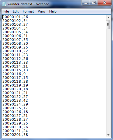
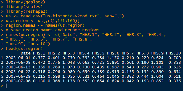
Open R, and read the CSV file with a header. Make sure your working directory is set where the data set is saved, and use the head() function to get an idea of what the data set contains.

Snapshot of Palladium Data

We see a date column with the format of "year-month-day", and the morning and afternoon prices in Hong Kong and New York, and only the morning price from London. We need to format the date column into a date type using as.Date(). Call str() to verify the type of the date column. Looking below, the date column is now in the date format.

Date Format

We will use the morning prices from Hong Kong ($Hong.Kong.8.30) because it has the most consistent, recent data out of the 5 price variables. For the recent date range, we aim for 2010 to present to capture the rise in palladium prices in 2011 in addition to the prices in late April 2014. After some exploring, we discover the starting index at row 1080.

Subset and Fix Value Typo

After we create the new subset, of the values from 2010 onward for the date and morning HK values, we discover the price range is slightly odd. There is a rather low anomaly price of 72. Using which.min() we locate the low price index at 131. To verify 72 is (in)correct, we look at the other variable locations at row 131, and realize that 72 was not the likely starting price. We impute a value of 723 at row 131 based on prices from other locations.

Now we can plot the palladium price get an idea of the data trend (and to see if it matches vaguely with the plot on Quandl). Add some color, axis labels, and title to the plot.

Plotting Palladium

We see the result below. Looks good, but this 'good' does not represent publishable material. This is simply raw R plot output.

Raw R Plot Output

Since this post is about turning a graph into a graphic, I made a few modifications to the R plot in Adobe Illustrator. First I used the direct selection tool to delete the plot borders, and to move the title, axis labels, and create the dashed lines as enhanced tick marks. Then I utilized the type tool to add text to highlight specific events on the time series, and created a sub-title explaining the graphic.

As a result of refining the plot through Illustrator, we see an improved visual with more pertinent information about South African, Ukraine, Russia, and palladium prices. The view can observe the events from the labels, and see the rise in palladium prices in response. However, this is not mean direct causation, but logically the effect of strikes/sanctions with production control and rising scarcity/prices makes sense. We want the visualization to invoke thought, and raise questions about the mechanisms behind the palladium price fluctuations. (Hopefully we will not encounter WWIII- and Putin is not shy about brinkmanship).

Stay tuned for more R analytics posts, and keep an eye out for additional visualization posts!


Thanks for reading,

Wayne
@beyondvalence
LinkedIn

Python: Converting CSV to XML and JSON

Hello Readers,


Today we will convert the common CSV (comma separated values) format into XML (extensible markup lanuage) and JSON (javascript object notation) formats in Python. The CSV file we will use was obtained from data scraping the weather underground website.

CSV Data

The CSV data has two elements in each row separated by a comma:
1. The date as 8 characters- 4 year, 2 month, 2 day
2. Temperature in Fahrenheit

CSV To XML

The XML format exists as self-defined tags, beginning with a XML declaration, specifying the XML version "1.0". There is a root element of <weather_data>, and a child element of <observation>, which also has a child element (sub-element) of <date> and <max_temperature>. The root and child elements make up the tree structure, and note that tags need to be closed as well.

XML Tree

To read the CSV file, we use the csv.reader() method, and set the delimiter to a comma. Then we create the XML file to which we will write the output, and write the XML heading and the root element.

Reading CSV and Writing XML

Now we iterate through the child elements of observations consisting of the date and maximum temperature. Recall that the date is in the first index and the temperature is in the second, with python index starting at 0. Remember to close the open tags afterwards, and close the XML document.

Observation Element and Closing Tags

We can see the results by opening the XML file, and opening it in a web browser, such as Google Chrome:

XML Output

Note how the root and child elements have arrows which we can minimize, and each observation is separate. Our XML formatting looks correct through Chrome. Although the output takes up more room than a CSV file, it is much more readable.

CSV To JSON

Javascript Object Notation is another format widely used to store and transfer data. It is quite different from XML, because it uses curly braces "{ }" for objects and brackets "[ ]" for arrays, instead of <tags> separating elements. The basic JSON format applied to our weather data is shown below. 

JSON Format

Even though we will not use the json module, I show it so you know it is there. Import the csv module to read our "wunder-data.txt" CSV file again, and write the "observation" object and begin an array with an open bracket. We start a rows_num variable at 0, and count to the max number of iterations (rows in the CSV file).

Import, Read and Write Data

Inside this array, we iterate our observation objects with name/value pairs with date and temperature. Incrementing the rows_num by 1 with each observation, if it reaches 354, we still want to include a comma after the closing curly bracket. But if it reaches 365, then we finish the observations and close the array and observations object.

Iterating Objects

Opening the JSON output in Google Chrome, we see a mess of name/value pairs. Clearly Chrome does not read plain JSON, but there are Chrome Apps available, such as JSONView.

JSON Output

Okay readers, we have covered much ground today with data formats. Both XML and JSON are widely used, knowing both will definitely allow you to utilize varied data sets. Stay tuned for more posts!


Thanks for reading,

Wayne
@beyondvalence

Python: Writing a Data Scraping Script

Hello Readers,


Today we will discuss data scraping, from a website's page source in HTML. Most of the times when we analyze data, we are provided the data, or are able to find the data through an online database. When we do, the data are usually arranged in a CSV/TSV format or as a convenient database waiting to be queried. Those types of data are known as structured data, and comprise only a fraction of the data available on the web.

To retrieve unstructured data  is usually a time consuming process if processed manually, since the data are not organized, or are large sections of text, such a server logs or Twitter tweets. They could even be spread over a number of web pages, for example, the maximum daily temperature in Fahrenheit for Buffalo, New York, starting from 2009. A screenshot highlighting the maximum temperature is shown below.

Weather History for Buffalo, NY

At 26 degrees, it was a cold New Years day in Buffalo. From the drop down options we can select January second to view that day's maximum temperature. You can imagine the time required to obtain the maximum temperature for each day in 2009. However, we can automate this process and skip the copy and paste/manual entry of the temperature through a Python script. We will use Python scrape temperature data from Weather Underground's website [1- Nathan Yau Flowing Data].

HTML Source

One thing to notice is the Buffalo historical weather page URL:

http://www.wunderground.com/history/airport/KBUF/2009/1/1/DailyHistory.html?req_city=NA&req_state=NA&req_statename=NA&MR=1

Even if we delete the URL after ".html", the page still loads. Also, we can spot the date in the URL, "/2009/1/1/". Remember this URL component, because it will be important when we automate the scraping with loops. Now we have discovered the range of URLs for daily weather in Buffalo in 2009.

http://www.wunderground.com/history/airport/KBUF/2009/1/1/DailyHistory.html
to ->
http://www.wunderground.com/history/airport/KBUF/2009/12/31/DailyHistory.html

In order for the Python script to scrape the data from the Weather Underground sites, we need to access the page source and see how the maximum temperature is coded. In Chrome, you can right click the page to view the page source in HTML.

HTML Page Source

Either through scrolling through the page or pressing Ctrl+F to find the text "Max Temperature", we can locate the desired temperature and the HTML tags around it. We spot the Max Temperature values enclosed by span class="wx-value" tags. Note that our target value is the third value enclosed by the span tag. The first two temperatures are the Mean Temperatures.

Python Script

We will use 2 libraries access the website and parse the HTML: urllib2 and BeautifulSoup. The first module provides standard functions for opening websites, and the second module is the crucial one. Created by Leonard Richardson, Beautiful Soup gives Python the power to navigate, search, parse, and extract parts of code we need.

After we import the two modules, we need to create the text file "wunder-data.txt" to which we will write the maximum temperatures.

Import and Open Text File

To automate the scraping process, we use loops to cover the months and the days in each month. Keeping in mind of the different days in each month, we use if and elif statements to check February, April, June, September, and November.

Looping

Inside the loops, we will print out the current date we are retrieving, and access the url with the current month (m) and day (d) using method urllib2.urlopen().

Print Current Date and Open Respective URL

After we opened the page, we pass it through BeautifulSoup(), and then use the soup.findAll() method to locate the tag "class: wx-value". Then we take the third value, [2], since the python index starts at 0, and bind it to our dayTemp variable. Next we format the month and day to be 2 characters by adding a "0" if required.

Using BeautifulSoup and Date Formatting

Now that we have the temperature in dayTemp, and proper date formatting, we create a timestamp with which we will write the dayTemp. This way, we can see the date of the retrieved maximum temperature.

Timestamp and Writing

Outside of the loops, we close the finished text file and print out a finished indicator. Below we have the output of the wunder-data.txt file. Observe the time stamp with 8 characters (4 for year, 2 for month, and 2 for day) followed by a comma and the temperature.

File Output

This post illustrates the basic concepts to data scraping:

1. Identifying the pattern (in URL / HTML source)
2. Iteration (script)
3. Storing the data (writing to file)

There are many other measures we could have included, such as the minimum temperature, or even a moving average of the maximum temperature in the script. The important thing is, do not let yourself be confined to using structured data in forms of CSV, TSV, or Excel files! Unstructured data are out there in large quantities, and it is up to you to retrieve, and clean them to be fit for analysis.


Thanks for reading,

Wayne
@beyondvalnence

R: Comparing Multiple and Neural Network Regression

Hello Readers,


Today we have a special competition between linear and neural network regression. Which will model diamond data best? Load the ggplot2, RSNNS, MASS, and caret packages, and let us turn R into a diamond expert. While the statistical battle begins, we can learn how diamonds are priced.


READY TO RUMBLE: Diamond Data

Here we will compare and evaluate the results from multiple regression and a neural network on the diamonds data set from the ggplot2 package in R. Consisting of 53,940 observations with 10 variables, diamonds contains data on the carat, cut, color, clarity, price, and diamond dimensions. These variables have a particular effect on price, and we would like to see if they can predict the price of various diamonds.

diamonds Data

The cut, color, and clarity variables are factors, and must be treated as dummy variables in multiple and neural network regressions. Let us start with multiple regression.

TEAM: Multiple Regression

First we ready TEAM: Multiple Regression by sampling the rows to randomize the observations, and then create a sample index of 0's and 1's to separate the training and test sets. Note that the depth and table columns (5, 6) are removed because they are linear combinations of the dimensions, x, y, and z. See that the observations in the training and test sets approximate 70% and 30% of the total observations, from which we sampled and set the probabilities.

Train and Test Sets

Now we move into the next stage with multiple regression via the train() function from the caret library, instead of the regular lm() function. We specify the predictors, the response variable (price), the "lm" method, and the cross validation resampling method.

Regression

When we call the train(ed) object, we can see the attributes of the training set, resampling, sample sizes, and the results. Note the root mean square error value of 1150. Will that be low enough to take down heavy weight TEAM: Neural Network? Below we visualize the training diamond prices and the predicted prices with ggplot().

Plotting Training and Predicted Prices

We see from the axis, the predicted prices have some high values compared to the actual prices. Also, there are predicted prices below 0, which cannot be possible in the observed, which will set TEAM: Multiple Regression back a few points.

Next we use ggplot() again to visualize the predicted and observed diamond prices from the test data, which did not train the linear regression model.

Plotting Predicted and Observed from Test Set

Similar to the training prices plot, we see here in the test prices that the model over predicts larger values and also predicted negative price values. In order for TEAM: Multiple Regression to win, TEAM: Neural Network has to have more wild prediction values.

Lastly, we calculate the root mean square error, by taking the mean of the squared difference between the predicted and observed diamond prices. The resulting RMSE is 1110.843, similar to the RMSE of the training set.

Linear Regression RMSE, Test Set

Below is a detailed output of the model summary, with the coefficients and residuals. Observe how carat is the best predictor, with the highest t value at 191.7, with every increase in 1 carat holding all other variables equal, results in a 10,873 dollar increase in value. As we look at the factor variables, we do not see a reliable increase in coefficients with increases in level value.

Summary Output, Linear Regression

Now we move on to the neural network regression.

TEAM: Neural Network

TEAM: Neural Network must ready itself as well. Because neural networks operate in terms of 0 to 1, or -1 to 1, we must first normalize the price variable to 0 to 1, making the lowest value 0 and the highest value 1. We accomplished this using the normalizeData() function. Save the price output in order to revert the normalization after training the data. Also, we take the factor variables and turn them into numeric labels using toNumericClassLabels(). Below we see the normalized prices before they are split into a training and test set with splitForTrainingAndTest() function.

Numeric Labels, Normalized Prices, and Data Splitting

Now TEAM: Neural Network are ready for the multi-layer perceptron (MLP) regression. We define the training inputs (predictor variables) and targets (prices), the size of the layer (5), the incremented learning parameter (0.1), the max iterations (100 epochs), and also the test input/targets.

Multi-Layer Perceptron Regression

If you spectators have dealt with mlp() before, you know the summary output can be quite lenghty, so it is omitted (we dislike commercials too). We move to the visual description of the MLP model with the iterative sum of square error for the training and test sets. Additionally, we plot the regression error (predicted vs observed) for the training and test prices.

Plotting Model Summaries

Time for TEAM: Neural Network so show off its statistical muscles! First up, we have the iterative sum of square error for each epoch, noting that we specified a maximum of 100 in the MLP model. We see an immediate drop in the SSE with the first few iterations, with the SSE leveling out around 50. The test SSE, in red, fluctuations just above 50 as well. Since the SSE began to plateau, the model fit well but not too well, since we want to avoid over fitting the model. So 100 iterations was a good choice.

Second, we observe the regression plot with the fitted (predicted) and target (observed) prices from the training set. The prices fit reasonably well, and we see the red model regression line close to the black (y=x) optimal line. Note that some middle prices were over predicted by the model, and there were no negative prices, unlike the linear regression model.

Third, we look at the predicted and observed prices from the test set. Again the red regression line approximates the optimal black line, and more price values were over predicted by the model. Again, there are no negative predicted prices, a good sign.

Now we calculate the RMSE for the training set, which we get 692.5155. This looks promising for TEAM: Neural Network!

Calculating RMSE for MLP Training Set

Naturally we want to calculate the RMSE for the test set, but note that in the real world, we would not have the luxury of knowing the real test values. We arrive at 679.5265.

Calculating RMSE for MLP Test Set

Which model was better in predicting the diamond price? The linear regression model with 10 fold cross validation, or the multi-layer perceptron model with 5 nodes run to 100 iterations? Who won the rumble?

RUMBLE RESULTS

From calculating the two RMSE's from the training and test sets for the two TEAMS, we wrap them in a list. We named the TEAM: Multiple Regression as linear, and the TEAM: Neural Network regression as neural.

Creating RMSE List

Below we can evaluate the models from their RMSE values. 

All RMSE Values

Looking at the training RMSE first, we see a clear difference as the linear RMSE was 66% larger than the neural RMSE, at 1,152.393 versus 692.5155. Peeking into the test sets, we have a similar 63% larger linear RMSE than the neural RMSE, with 1,110.843 and  679.5265 respectively. TEAM: Neural Network begins to gain the upper hand in the evaluation round.

One important difference between the two models was the range of the predictions. Recall from both training and test plots that the linear regression model predicted negative price values, whereas the MLP model predicted only positive prices. This is a devastating blow to TEAM: Multiple Regression. Also, the over prediction of prices existed in both models, however the linear regression model over predicted those middle values higher the anticipated maximum price values.

Sometimes the simple models are optimal, and other times more complicated models are better. This time, the neural network model prevailed in predicting diamond prices.

Winner: TEAM: Neural Network

Stay tuned for more analysis, and more rumbles. TEAM: Multiple Regression wants a rematch!

Thanks for reading,

Wayne
@beyondvalence
LinkedIn
rumble

Visualizing Google Flu Trends Part 2

Hello Readers,


This post continues the visualization of flu trends from Google. Last time we plotted the flu time series for 50 states from 2003 to 2013. Here we will visualize the flu trends through 10 regions set by the Department of Health and Human Services (HHS). We shall enlist the aid of the melt() function from the reshape2 library.

So load ggplot2, scales, and reshape2 in R, and let us get started!

10 HHS Regions

Recall from the previous flu trends post, that the data was obtained from the Google Flu Trends site. The CSV file includes influenza like illness percentages from doctor visits for 50 states, District of Columbia, 97 major cities and 10 HHS regions. Since we already visualized the 50 states, we turn to the 10 HHS regions.

Flu Data in U.S. Regions

Last time we used a custom function to pull data from each column into 1 column. Then we bound a respective column with the 50 state names. Likewise, the date values were repeated 50 times, for a total of 3 columns. The original saved region names are shown below, along with the states they contain.

Original Region Names with States

However, there is (almost always) a more efficient way. In the reshape2 library, there exists a function which will arrange all the desired values into one column from multiple columns. Simply specify which variable to keep constant, and the melt() function will create variable column identifying the value column.

Melted Flu Trends in U.S. Regions

Now we are ready to visualize the flu data by region.

Creating the Visuals

Using ggplot(), we specify the Date on the x axis, and the value on the y axis. Furthermore, we use facet_wrap() to stratify by variable (HHS regions) into 10 plots, 2 columns of 5.

Plot Code

This yields the plot below:

Like we confirmed in the last post, here we also see dramatic peaks in all regions from 2003-2004, and 2009-2010. HHS region 6, which includes Arkansas, Louisiana, New Mexico, Oklahoma, and Texas has higher consistent peaks than the other 9 regions.

We could have plotted the 10 regions in one plot, however, the lines would be difficult to differentiate:

Plot Code

Looking at the plot below, we observe multiple colors, each a region, and peaks in each region occur within a similar time window. All the lines in one plot makes it difficult to evaluate each time series individually, but allows relative comparison between regions.

Again we encounter an alternative method to writing a custom function. The melt() function rearranges a data.frame for us. And that concludes this post. Stay tuned for more data analysis!


Thanks for reading,

Wayne
@beyondvalence
LinkedIn