P1.7: Exploring Power View Reports in Excel

This post explores the Reports produced by Power View in Excel 2013. The data we will use is from the AdventureWorks dataset, which is in the Chapter 1 workbook from the Alberto Ferrari PowerPivot book.

Creating a Power View Report

Similar to a Dashboard we created in P1.5, Power View in Excel can construct a report which can convey data to the reader, but with more visualization capabilities. Reports from Power View require minimal mouse clicks to embellish and offers Excel users a graphical data exploration tool. PivotTables allow Excel users to explore data using tables, whereas Power View allows us to explore the data graphically in a simple charting environment.

Power View works through the Data Model and not Excel tables, so if you add tables to the Power View report, they will be added to the Data Model. Make sure you have MS Silverlight installed for Power View to work.

Click on the Power View button on the Insert tab in Excel. We will create a new Power View report, so click OK when Create a Power View sheet is selected.

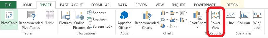
Fig. 1: Power View button

Now we have a Power View report from which we can add fields. Start by clicking on the report and then selecting the ProductCategory and SalesAmount fields from the Sales table from the Power View Fields on the right pane. You can also add an appropriate title to the top of the Report, and this particular one I will name "Sales by Category and Geography".

Fig. 2: Product Category and Sales in Power View Report

Now suppose you would like to show more information, such as sales by geographical region. To start another table, click on an empty area in the Power View Report. If you add more fields with the previous table open, then the fields will be added to the previous table. Select the fields of TerritoryCountry and SalesAmount in the Sales table. This will display a table showing the country and the sales.

Fig. 3: Country and Sales table in Power View Report

Looking at the Sales by Country in a tabular format is not exactly visually appealing. However, we can portray the geographic data on a map, which will enhance the analysis visually. An internet connection is required to map the data. With the TerritoryCountry table selected, click on the Map button in the Design tab, and the table is converted into a map chart showing SalesAmount as circles over the respective country.

Fig. 4: Map Chart of TerritoryCountry and SalesAmount

We can re-size and zoom in or out of the map to display the area we would like to exhibit on the report. The product category table can also be converted into a visually appealing format as a chart by selecting the Column Chart button in the Design tab.

Fig. 5: Column Chart of ProductCategory and SalesAmount

Adding Filters to the Power View Report

While creating a report in Power View, we can also add a filter to aid in analyzing the data. Let us include the Office and SalesManager fields as filters to the report to see the stratified data graphically. Start by adding the Office and SalesManager as two tables on the above report.

Fig. 6: Office and SalesManager Tables on the Sales Report

Now that we have the two tables added, we can change them to what Excel calls a Slicer. With the desired table selected, click on the Slicer button in the Design tab.

Fig. 7: Office Table as Slicer in the Sales Report

In Figure 7, the Office table is now a Slicer, or filter, and the SalesManager table is selected ready to be converted into a Slicer as well, with the highlighted Slicer button. With both fields as Slicers, we can now stratify the Office and SalesManager fields to show data on the Sales Report which only relate to that specific selection in the field. For example, we can select the Seattle office and Alberto Ferrari as the sales manager. The data on the Power View report would only reflect the Sales by the Seattle office and those under the sales manager, Alberto Ferrari.

Fig. 8: Sales in the Seattle Office with Alberto Ferrari as Sales Manager

Filters and slicers allow us to view the data under different field selections. In the Power View Report, the chart is updated automatically with the selected filter, which enables fast and efficient data analysis. We can clear the filters by clicking on the Eraser button on the top right-hand corner of the filter table, shown in Figure 9 below.

Fig. 9: Clear Filter Button

To conclude, Excel charts allow large areas customization, with many options to choose. In contrast, Power View charts give the user the ability to visualize the data and spot patterns from the charts with minimal effort in creation.


Thanks for reading,
Wayne