P1.3: Using a PivotTable to Query a Data Model- Excel 2013

Hello Reader. Here you will learn how to query a data model created in the past post with a PivotTable in Excel 2013.

Querying a Data Model

Start by opening the PivotTable workbook in Chapter 1 with the AdventureWorks dataset in Excel. To query, or use the data model containing the Sales and SalesManagers tables, you select the Insert tab and click on the PivotTable button.

Fig. 1: PivotTable Button on Insert Tab

A dialogue window appears showing options for creating a new PivotTable. In the first section, select Use an external data source and click the Choose Connection button for locating more data.

Fig. 2: Creat PivotTable Options

You can select the desired data model in the workbook by looking under the Tables tab and click Open, shown in the figure below. Also, you can note that individual tables in the workbook can be selected as well, which could be added to the data model by checking the Add this data to the Data Model box at the bottom of Figure 2.

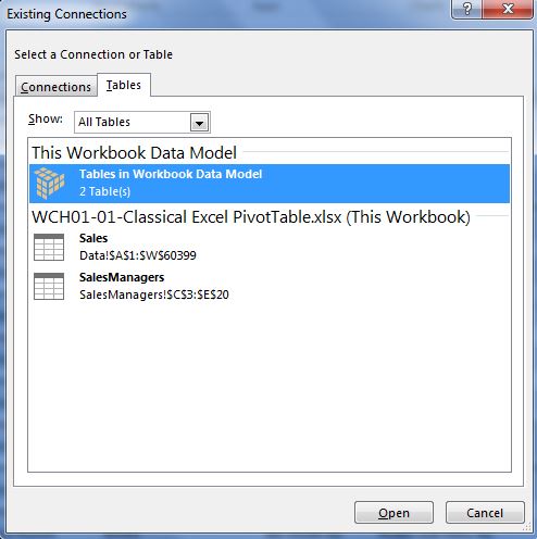Fig. 3: Data Model in Connections Window

Now you have a PivotTable from which you can select fields to query in the report.

Fig. 4: A New PivotTable

Note
When you create a PowerPivot data model, it is different and distinct from a Excel table. The table is not converted into a PivotTable when you add data from the table to the data model. Instead, Excel creates a PivotTable for the table and links them, so if the table data is modified, it reflects on the updated PivotTable. Once updated, the data model is updated as well. Essentially, the data is in the Excel table, and in PowerPivot.

Thanks for reading,
Wayne