Predictive Modeling: Decision Trees and Recursive Partitioning in R

A Decision Tree

Hello Readers,


Sometimes we encounter situations where we would like to know the outcome or result of an event given a few factors or variables. In other words, we would like to predict the result. R allows us to create models given the available information to predict what we want to know.

This post will discuss a predictive analysis method, decision trees- a type of non-parametric modeling.


Open R and let us get started!

The Question and the Data

Before approaching the first steps in predictive analysis, keep in mind the result has to answer the question, and the results depends on the analysis we conduct. By initially asking the right question about the data, we can derive a valid answer from the subsequent analysis. Knowing the data, and knowing what we want to discover about the data is an important first step before beginning analysis. So let us look at the dataset.

We will be using the iris dataset already in R. Go ahead open R and call str() on iris to get an idea of the variables in the data.frame. The output is shown below.

str(iris)

Iris is composed of 150 observations with 5 variables which describe the various attributes of the iris plant species. We can plot a few variables by Species to get an idea of the correlation.

Iris Measures Plot

Immediately we can consider whether the first four variables can accurately predict the Species variable. Can we tell which species of iris a particular plant belongs to with some sepal and petal measurements? Let us find out.

Creating The Tree

Start by importing the party package to use decision trees with library(party). Next we will create an index with sample() to separate the data into 70% training data and 30% test data (the seed is 1234 to reproduce the pseudo-random sampling). 

Training and Test Data

Str() the d.train data to verify, and we see that there are 112 observations in d.train, out of the 150 in the original, which is what we wanted (a little over 70%, but it is random).

Next we designate the predictor variables as Sepal.Length, Sepal.Width, Petal.Length, Petal.Width, and the response variable as Species. Then ctree() function creates a binarytree object, and we store it as iris.tree. To see how the iris.tree model compares to the actual species, check it a table:

Iris Tree Formula and Table

We see that all of the setosa species were classified, but versicolor and virginica had 1 and 3 off, respectively- not too shabby. The plot of the iris decision tree is shown below. The petal length was the first chance node, which branched to petal width, then petal length again, creating 4 groups.

Iris Decision Tree

And now that we have 'trained' the data to create the tree classifier, we can predict the the iris species in the d.test data using the predict() function.

Predictions on Iris Test Data

We observe that the setosa and versicolor were predicted well but again, we see that the model missed 2 observations as versicolor when they were in fact, virginica.

Creating Another Tree: Recursive Partitioning

R has several decision tree packages and we will use the rpart package for the next tree. Use library(rpart) to load rpart, and also load the mboost package as well for the bodyfat dataset. Call the str() function on the bodyfat dataset.

Bodyfat Dataset

We will concentrate on predicting the DEXfat levels with the other variables. Again, we will create a separate test and training data sets, so create an index and then use it to create the data sets.

Training and Test Data Sets

Use the age, waistcirc, hipcirc, elbowbreath, and kneebreadth as the predictor variables for DEXfat. In the rpart() function, control the  size of the node to split in the tree by declaring a node to have at least 10 observations.

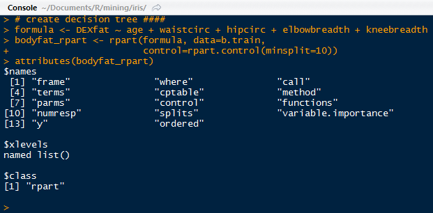Bodyfat Tree and Attributes

The bodyfat_rpart is a list containing all the attributes of the decision tree. Next, print the complexity parameter by printing the $cptable in the list. If a split does not decrease the overall lack of fit by a factor of cp, then the split will not occur. The default method uses anova splitting, so the R-squared must increase by cp each step.

Complexity Parameter Table

Next, we can print the tree as shown below. As you can see, it was split 7 times, first by wasitcirc, then by hipcirc and waistcirc and so on.

Bodyfat Tree

To visualize the tree, we use the plot() function, and add the text labels using text() like below:

Plot(), Text(), and the Bodyfat Tree

After which, we can select the tree with the minimum prediction error, from the cptable. The code is illustrated below, where the index of the minimum value of xerror in the cptable is assigned to opt and the respective CP value is passed as the cp value in the prune() function. That yields a tree with a specified prediction error:

Pruning a Tree

Again, we can visualize the newly pruned tree. Notice any differences between the previous tree and the pruned tree?

The Pruned Tree

Yes, the pruned tree does not have the node split from the 4th leaf from the left, instead it ends in the leaf. The xerror from the cp table for that split was greater than the xerror of the previous # 6 split so the pruned tree only has branches up to the lowest prediction error.

Checking the Predictions

Lastly, we will check how the pruned tree predicts DEXfat in the test data set after being fitted to the training data set. Use the predict() function to predict the DEXfat in the b.test data set, and plot the observed vs the predicted to see how close the values are.

DEXfat Prediction and Plot Code

After drawing the perfect prediction line y=x, with abline(), we can see how the predicted values compare with the observed. Note that the values fall generally along the line. The values above the line indicate an over prediction of the values, and those below the line are under predicted.

Predictions vs Observed DEXfat Values

Also, we see that the predicted values come in single values for a ranged of observed values- the values increase by fixed amounts. That is due to the tree classification giving the same predicted value for a set of predictor variables. The observations each leaf will have the same predicted value.

As you can see, decision trees are useful for non-parametric prediction modeling. However, decision trees can over fit the data, so caution must be used, and tree pruning with a predefined acceptable prediction error must be considered for a robust analysis.


Stay tuned for more on prediction modeling and other statistical topics in R!


Thanks for reading,


Wayne
@beyondvalence