Predictive Modeling: Creating Random Forests in R

Hello Readers,

Welcome back to the blog. This Predictive Modeling Series post will cover the use of Random Forests in R. Before we covered decision trees and now we will progress a step further in using multiple trees.

Click here to read Leo Breiman's paper for random forests.


Load the randomForest library package in R, and let us begin!

Iris Data

We will use the familiar iris data set found in previous posts as well. To remind us what we are working with, call head() on iris. 

Load randomForest and iris data

We are looking at four variables of the flowering iris plant and the fifth variable indicates the species of the flower. Now we can separate the data into a training set for the random forest and a testing set to determine how well the random forest predicts the species variable.

First sample 1 and 2 from the row number of the data set. We set the probability of 1 at 0.7 and 2 at 0.3 so that we get a larger training set. Then we assign the respective subsets of iris to their training and testing sets.

Creating Training and Test Data

Now that we have our data sets, we can perform the random forest analysis.

Random Forest

The Random Forest algorithm was developed by Leo Breiman and Adele Cutler. Random Forests are a combination of tree predictors, such that each tree depends on a random vector sampled from all the trees in the forest. This incorporates the "bagging" concept, or bootstrap aggregating sample variables with replacement. It reduces variance and overfitting. Each tree is a different bootstrap sample from the original data. After the entire ensemble of trees are created, they vote for the most popular class.

With the randomForest package loaded, we can predict the species variable with the other variables in the training data set with 'Species ~ .' as shown below. We are going to create 100 trees and proximity will be true, so the proximity of the rows values will be measured.

iris Random Forest

See that we have results of the random forest above as well. The 'out of bag' estimate is about 4.59%, and we have the confusion matrix below that in the output. A confusion matrix, otherwise known as a contingency table, allows us to visualize the performance of the random forest. The rows in the matrix are the actual values while the columns represent the predicted values.

We observe that only the species setosa has no classification error- all of the 37 setosa flowers were correctly classified. However, the versicolor and virginica flowers had errors of 0.057 and 0.081 respectively. 2 versicolors were classified as virginica and 3 virginicas were classified as versicolor flowers.

Call attributes() on the random forest to see what elements are in the list.

Attributes of iris Random Forest

Visualizing Results

Next we can visualize the error rates with the various number of trees, with a simple plot() function.

plot(rf)

Though the initial errors were higher, as the number of trees increased, the errors slowly dropped somewhat over all. The black line is the OOB "out of bag" error rate for each tree. The proportion of times of the top voted class is not equal to the actual class is the OOB error.

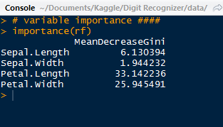
We observe which predictors were more important with the importance() function. As we can see, the most important variable was Petal.Length.

Important Predictors

Using the varImpPlot() function, we can plot the importance of these predictors:

For our most important variables for classification are Petal.Length and Petal.Width, which have a large gap between the last two sepal variables. Below we have the species predictions for the iris test data, obtained by using the prediction() function.

Iris Test Contingency Table

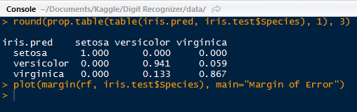
We see again that the setosa species performed relatively better than the versicolor and virginica. With the prop.table() function nested outside of the table() function, we can create a table for the proportions. Versicolor performed second best with 94% correct and virginica with 86%.

Proportion Table with Plot Code

We can go ahead a create a plot of the margin of error. The margin for a particular data point is the proportion of votes for the correct class minus the maximum proportion of votes of the other classes. Generally, a positive margin means correct classification.

Margin of Error Plot

We can see that as the most of the 100 trees were able to classify correctly the species of iris, although the few at the beginning were below 0. They had incorrectly classified the species.

Overall, the random forests method of classification fit the iris data very well, and is a very power method of classifier to use in R. Random forests do not overfit the data, and we can implement as many trees as we would like. It also helps in evaluating the variables and telling us which ones where most important in the model.

Thanks for reading,


Wayne
@beyondvalence