Loading...

Monday, December 23, 2013

Predictive Modeling: Decision Trees and Recursive Partitioning in R


A Decision Tree
Hello Readers,


Sometimes we encounter situations where we would like to know the outcome or result of an event given a few factors or variables. In other words, we would like to predict the result. R allows us to create models given the available information to predict what we want to know.

This post will discuss a predictive analysis method, decision trees- a type of non-parametric modeling.


Open R and let us get started!


The Question and the Data


Before approaching the first steps in predictive analysis, keep in mind the result has to answer the question, and the results depends on the analysis we conduct. By initially asking the right question about the data, we can derive a valid answer from the subsequent analysis. Knowing the data, and knowing what we want to discover about the data is an important first step before beginning analysis. So let us look at the dataset.


We will be using the iris dataset already in R. Go ahead open R and call str() on iris to get an idea of the variables in the data.frame. The output is shown below.


str(iris)

Iris is composed of 150 observations with 5 variables which describe the various attributes of the iris plant species. We can plot a few variables by Species to get an idea of the correlation.

Iris Measures Plot

Immediately we can consider whether the first four variables can accurately predict the Species variable. Can we tell which species of iris a particular plant belongs to with some sepal and petal measurements? Let us find out.


Creating The Tree


Start by importing the party package to use decision trees with library(party). Next we will create an index with sample() to separate the data into 70% training data and 30% test data (the seed is 1234 to reproduce the pseudo-random sampling). 


Training and Test Data

Str() the d.train data to verify, and we see that there are 112 observations in d.train, out of the 150 in the original, which is what we wanted (a little over 70%, but it is random).

Next we designate the predictor variables as Sepal.Length, Sepal.Width, Petal.Length, Petal.Width, and the response variable as Species. Then ctree() function creates a binarytree object, and we store it as iris.tree. To see how the iris.tree model compares to the actual species, check it a table:


Iris Tree Formula and Table

We see that all of the setosa species were classified, but versicolor and virginica had 1 and 3 off, respectively- not too shabby. The plot of the iris decision tree is shown below. The petal length was the first chance node, which branched to petal width, then petal length again, creating 4 groups.


Iris Decision Tree

And now that we have 'trained' the data to create the tree classifier, we can predict the the iris species in the d.test data using the predict() function.


Predictions on Iris Test Data

We observe that the setosa and versicolor were predicted well but again, we see that the model missed 2 observations as versicolor when they were in fact, virginica.


Creating Another Tree: Recursive Partitioning


R has several decision tree packages and we will use the rpart package for the next tree. Use library(rpart) to load rpart, and also load the mboost package as well for the bodyfat dataset. Call the str() function on the bodyfat dataset.


Bodyfat Dataset

We will concentrate on predicting the DEXfat levels with the other variables. Again, we will create a separate test and training data sets, so create an index and then use it to create the data sets.


Training and Test Data Sets

Use the age, waistcirc, hipcirc, elbowbreath, and kneebreadth as the predictor variables for DEXfat. In the rpart() function, control the  size of the node to split in the tree by declaring a node to have at least 10 observations.
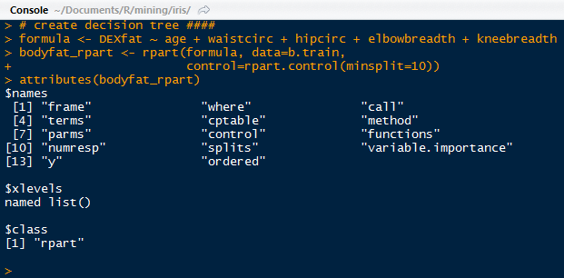

Bodyfat Tree and Attributes

The bodyfat_rpart is a list containing all the attributes of the decision tree. Next, print the complexity parameter by printing the $cptable in the list. If a split does not decrease the overall lack of fit by a factor of cp, then the split will not occur. The default method uses anova splitting, so the R-squared must increase by cp each step.


Complexity Parameter Table

Next, we can print the tree as shown below. As you can see, it was split 7 times, first by wasitcirc, then by hipcirc and waistcirc and so on.


Bodyfat Tree

To visualize the tree, we use the plot() function, and add the text labels using text() like below:


Plot(), Text(), and the Bodyfat Tree

After which, we can select the tree with the minimum prediction error, from the cptable. The code is illustrated below, where the index of the minimum value of xerror in the cptable is assigned to opt and the respective CP value is passed as the cp value in the
prune() function. That yields a tree with a specified prediction error:


Pruning a Tree

Again, we can visualize the newly pruned tree. Notice any differences between the previous tree and the pruned tree?


The Pruned Tree

Yes, the pruned tree does not have the node split from the 4th leaf from the left, instead it ends in the leaf. The xerror from the cp table for that split was greater than the xerror of the previous # 6 split so the pruned tree only has branches up to the lowest prediction error.


Checking the Predictions


Lastly, we will check how the pruned tree predicts DEXfat in the test data set after being fitted to the training data set. Use the predict() function to predict the DEXfat in the b.test data set, and plot the observed vs the predicted to see how close the values are.

DEXfat Prediction and Plot Code

After drawing the perfect prediction line y=x, with abline(), we can see how the predicted values compare with the observed. Note that the values fall generally along the line. The values above the line indicate an over prediction of the values, and those below the line are under predicted.

Predictions vs Observed DEXfat Values

Also, we see that the predicted values come in single values for a ranged of observed values- the values increase by fixed amounts. That is due to the tree classification giving the same predicted value for a set of predictor variables. The observations each leaf will have the same predicted value.

As you can see, decision trees are useful for non-parametric prediction modeling. However, decision trees can over fit the data, so caution must be used, and tree pruning with a predefined acceptable prediction error must be considered for a robust analysis.


Stay tuned for more on prediction modeling and other statistical topics in R!


Thanks for reading,


Wayne
@beyondvalence

Monday, December 16, 2013

Querying Trends with Twitter API Using Python


Hello Readers,

Hope you guys are keeping warm! Today we will be talking about mining the rich metadata of Twitter through their Twitter REST API v1.1 by using Python (I will use IPython 2.7.5 and the python twitter library). Specifically, we will look at trending topics. (For Part 2: Tweets, click here).

Let us begin.


For Starters


A Twitter account (my handle is @beyondvalence) is required to obtain the proper authorization keys to access the Twitter API. Go here to use your Twitter account to obtain developer credentials and keys. OAuth offers a solution for apps to access user Twitter data without requiring users to share sensitive information such as passwords. A sample of the Twitter development page with the OAuth keys is shown below.


Twitter OAuth Keys
Next, install the twitter library into Python by using the pip install in the command console. 


In IPython 


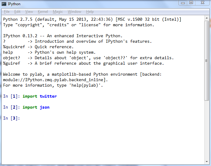
In the python IDE, we now can import twitter and json (JavaScript Object Notation) libraries, simple enough.


Import Twitter and JSON

Next, we define the OAuth keys as consumer, consumer_secret, oauth_token, and oauth_token_secret. Using these keys, create an OAuth authorization object, such as auth, shown below (line 4). Then auth is passed to class Twitter to issue queries to the Twitter API.


Gained Twitter API Query Access

The Twitter object print-out in line 5, above, indicates that we have used OAuth credentials to gain authorization to query Twitter's API.


Querying Trend Topics


Moving along! Now that we are authorized, we can issue a request. A common measure of topics in the Twitterverse is compiled in trends- which are popular tokens such as key words, handles, or hashtags. We can request the current trending topics on Twitter (as of this blog post writing in mid December).

Yahoo has developed an unique, non-repetitive way to index places by using the WOE (What On Earth) identifier. So we can use these WOE IDs to constrain our queries to Twitter, by using the 1 and 23424977 IDs for the entire world and the US, respectively. This is shown below. (The id requires an underscore to denote it as a query string parameterization.)


Twitter Trends Output

The result is a lot of text, much of it semi-readable at best. Deciphering the output is made easier to view by using JSON formatting.


JSON, a Data Exchange Format


We imported the json library at the beginning, and now we can print the API output in JSON. Do this for the trends in the US, by using print json.dumps(). This is shown below.


API Output JSON Format

Much better! As we can see some trending topics in the US are:


  • #LastMinuteGifts (Makes sense, being in the Holiday shopping season)
  • #SOTV
  • #AskHartnell
  • Christmas (just around the corner)
  • 22 Jump Street (a comedy movie)
And trending topics in the world include:

  • #YeterArt
  • #MilletinVekiliHakan
  • #SessizSakinTakiple
  • #TMP332
  • Julie Plec Needs Kol


Note: Twitter Rate Limits

Twitter has rate limits on applications constraining the number of requests one can make to an API at 15 requests in a 15 minute time window for trends. It is not a big concern considering the trends are updated every 5 minutes anyways.

Later posts will discuss more Twitter metadata, like tweets! Stay tuned for Part 2, Querying Tweets!

Thanks for reading &
Have a wonderful Holiday! 


Wayne
@beyondvalence

Thursday, December 12, 2013

Visualizing Twitter Tokens- Hashtags, Smileys and URLs in R


Hello Readers!

Tweet, Tweet!
Welcome back to the blog. Today we will discuss how to visualize Twitter tokens trends in tweets, specifically:


The data was obtained from the infochimps site, where they also host data sets for other platforms. For analysis I will be using RStudio.

Let us get started.


The Loading


Unpacked Zip File Content
Once we have downloaded and unzipped the 'tokens by month' data set, we can go ahead a read the tsv file (tab separated values) into R. Use the str() function to get an idea of the data structure.


Reading in Total Tokens by Hour tsv
Looking at the structure, we see that there are 3 columns with 67,992 observations consisting of "tweet_url", "smiley", or "hashtag". The X column denotes the 4 digit year, month, day, and hours in 24 hour format, followed by the count in the X1 column. Use the table() function to determine how many token measures we have of each, and also to check for spelling errors.


Token Measures
We see there are 18,401 hashtag measures, 25,137 smiley measures, and 24,454 tweet_url measures. Keep in mind these are not counts- they are just the number of times the tokens were measured in the data set. The actual counts are in column 3, X1. To obtain the total counts for each measure, we use tapply() to apply a function by index. The totals are shown above, with tweet_urls coming in top at 167,819,007! It seems that people are tweeting more internet links than hashtags and smileys put together.


The tokens() Function


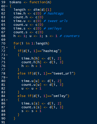
Next we write the tokens() function. Keep in mind of the variables we have to track when we separate the all the information pertaining to the three different tokens. At the same time, I want to convert the dates into an usable Date.Time format. Putting it together, the result will be a list containing the date and count of the hashtag, smiley, and tweet_url tokens.

The first part of the function is shown below.


Token Function Part 1
 We start the function by initializing the variables we need to keep track of and using counters to progress the variables along through each successive record (h, u, and s) of their respective time and count variables in the for loop. We take the pertinent data from each type of token into their own variables to put in a list. 

Next, we take the date variables and convert them into Date.Time format using the strptime() function, shown below. Afterwards, we create the list and instruct the function to return the tokens list. Now run the tokens () function.


Token Function Part 2
Finally, use the completed tokens() function to create the t.tokens list.


The Plotting


Now that we have the tokens in a convenient list, we can visualize the token trends with a plot. Naturally, use the plot() function, a sample method is show below.


Plotting the Hashtag Count
 The second section will create the x axis labels consistent with the Date.Time values in the t.tokens$count.h variable. It will plot the year and month for better readability.

Hashtag Count Plot

We will add the two other tokens next using the lines() function. And to finalize the plot, we will add a legend to interpret which line is which token.


Adding Smiley and URL Count Lines

Now we have the finished plot!

Plot of All Three Token Counts Over Time

Note that starting in January of 2009, user activity, especially in URL content are beginning to spike above the previous background levels. Observe that drastic spikes in URL counts in July and October of 2009 also coincided with hashtag and smiley counts as well. The increases in content can be attributed to the increased in Twitter users, starting in 2009. 

Stay tuned for more Twitter analysis!

Thanks for reading!


Wayne

Tuesday, December 10, 2013

Importing Data into a Database Engine, SQL Server 2012

Hello Readers!

Welcome back. We need data to be able to query tables. So today we will walk through how to import data into a Database Engine in SQL Server Management Studio 2012. Click here for more info on SSMS 2012. 

Let us get started!


The Setup


First, open SQL Server Management Studio (SSMS). We are greeted with a dialogue box to connect to a server. I will use Windows Authentication to connect to my local server. 


Connect to a Server
After we have connected, we see the Object Explorer to the left of the screen. The Server will show a green arrow to indicate a successful connection. The Object Explorer allows us to view and manipulate the different utilities, tools, and capabilities in SSMS. The expanded explorer box is shown below. Note the green 'good to go' arrow by the server name.


Connection Established


Importing the Data


Now we need to import the data. It would be helpful if we had the target data already on the computer, and in this case, we will be importing the familiar AdventureWorks database which exists as an Access database file. We can also import it as an mdf (mirror disk file) from this link.

Start by right clicking the database to where the data will be imported. Now from Tasks, click Import Data... towards the bottom.


Import Data Button

In step, we are in the SQL Server Import and Export Wizard. As shown below. Select the appropriate data source and locate the file on the hard drive:

Select the Data Source and Location


After choosing the input specifications, we need to choose the output Destination. I will import the data into the POWER (short for PowerPivot) database.

Choosing the Destination

And then for the nitty-gritty of specifying which tables to copy. We have two options: manual selection or SQL query. Select either, I will select manual because I will be copying all the data.


Specify Which Selection Method

After which, we can check the boxes of the tables we require. Clicking the box at the top left will select all of the tables. Click Next.

Selecting Tables

We are then given a review of the selected tables before they are imported into the database. The table attributes and types are shown to verify the correct tables have been selected, below.

Data Type Review
Clicking Next and Finish, we now have the tables in the POWER database. The Object Explorer below reflects the newly imported tables.

Object Explorer with New Tables

And with the new query window open, we can now query tables that we require!

Blank Query Window

That concludes this post on how to import data into a database in SQL Server Management Studio 2012. Future posts will include SQL querying and use of the SSMS Analysis Services to analyze the data. Also, I will include a post on using R to connect to SQL Server to retrieve tables. Please look forward to the new posts!


Thanks for reading!


Wayne

Monday, December 9, 2013

P4.4: Data Modeling in PowerPivot: Relationship JOIN Types

Hello Readers,

In this post we will continue our discussion (from P4.3) on the types of JOINS we can use when creating relationships, especially through SQL queries. As usual, we will be using the AdventureWorks dataset from the Ferrari book. Let us begin.


JOINS


When we join two tables together, we have to determine what we want in the resulting table. Whether we need all of the rows in a specific table or just the matches in both, specific joins enable us to manipulate the merging of two tables in different ways. Subsequently, the left and right tables we choose have positional distinctions when we select a specific type of join method. 


Detailed below are the different types of joins. (Diagrams from stackoverflow.)


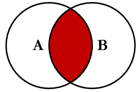
INNER JOIN


When two tables are joined using an inner join, only the rows in table A which match the related rows in table B will be included in the resulting table. This is why in the previous post, P4.4, the joining of DimProduct with 606 entries and DimProductSubcategory tables yielded only 397 entries. There were only 397 product rows which had both an EnglishProductCategoryName and EnglishProductSubcategoryName.


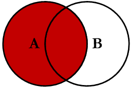
LEFT OUTER JOIN


The left join is similar, but includes the all the entries in table A, and records NULL for entries in table A with no corresponding entries in table B.


RIGHT OUTER JOIN


The right outer join is the mirror image of the left outer join. All entries in Table B will be included, and those rows without a corresponding row in Table A will show NULL.


FULL OUTER JOIN


Next is the full outer join where both Tables A and B are preserved, with entries in Table A with none in B, and entries in Table B without entries in A will show as NULL.


LEFT EXCLUDING JOIN


Using left exclusion join we can modify the join to yield only entries in Table A which do not match in the right Table B.


RIGHT EXCLUDING JOIN


Likewise with a right excluding join, the all entries in Table will be included except for those which have corresponding entries relative to entries in Table A.


Here is a helpful link!


Thanks for reading,


Wayne Liu

R: Regex Telephone Number Matching

Hello Readers,


Firstly, here is an encouraging message from President Obama, calling for more students to learn code! Hooray, SCIENCE!


Now back to the post. Here we shall discuss using regular expressions to match North American telephone numbers in RegExr. For matching text from HTML5, check out this post.

Usual telephone numbers include a three digit area code followed by a seven digit number sequence, which can be separated by hyphen, period or even spaces. Sometimes the area code can be enclosed in parenthesis as well. So how do we match and extract the numbers that we require? So we turn to the flexibility of Regular Expressions to describe the target string we want to match. We will be using RegExr program, found here. Let us get started.


RegExr


The picture of the RegExr window, above, shows a variety of telephone numbers, some separated with hyphens, some with periods, and others just with spaces. So how can we match the digits in the phone numbers? To demonstrate, we can first use:

1. Literal Strings

  By using the actual numbers, we can manually match the telephone numbers. For example, if we type 498, then RegExpr matches the sequence of digits 498 twice, as shown below.


RegExpr Matching 498

2. Shorthand

  By using the power of regular expressions, we can incorporate shorthand, which is a special type of character. A backlash lowercase d denotes any digit. The opposite is true when the d is capitalized to D, as any character that is not a digit is matched, such as hyphens, periods, parenthesis, etc. Both are shown below.


Matches Any Digit- Shorthand
And the reverse (conveniently the capitalized letter D):

Matches Any Non-Digit- Shorthand
3. Quantifiers

Since telephone numbers follow a pattern of 3 digits, 3 digits, and 4 digits, we can tell the match to loop for a certain amount of times by using a quantifier. For example, using curly brackets {n} to surround a number after a regular expression will instruct RegExr to match that expression n times. This is shown below, as \d (any number) is matched exactly three times. Note how in the last set of 4 digits, only the first 3 are matched.


Shorthand Matching with a Quantifier
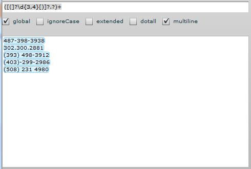
To match the set of 4 numbers as well, we can use {n1, n2} as a quantifier where RegExr will match expression from the range n1 to n2. Additionally, the quantifier ? matches 0 or 1 of the preceding token, whereas the + will match 1 or more. The asterisk * will match 0 or more times.


More Quantifiers- It Works!
The ? after both parenthesis allow them to match when they are and are not there, so it will match the area code as well as the other digits in the phone number. The digit sets are set to match {3, 4} three to four times, and the optional period will match any character, whether it be a hyphen, period, or white space. Then the whole expression has to match at least once or more with the + sign.
4. Putting It Together


However, there are many different ways to match a specific string. Below is another method which uses anchors.

Simply put, anchors do not match a specific character in the string, it matches the position. So while we can use the carrot sign, ^, to match the beginning of a line, it will not return any value without an expression. Likewise, the $ matches the end of a line.

See how the ^ and the $ constrain the first set of tokens to match the area code with or without the parenthesis at the start of the line, and that the last set of 4 digits have to end at the end of the line. The non-digits are matched with the \D token.


Another Method Using Anchors

Now we have seen the power and flexibility of regular expressions and how it can match numbers and different symbols. They will be very important when analyzing text data as well, especially making sense of data in HTML5 format.

We will continue to solve more regular expression problems in future posts. Stay tuned!
As always, thanks for reading,


Wayne