KDD Cup: Profit Optimization in R Part 2: Decision Trees

Hello Readers,

This post continues the Knowledge Discovery and Data mining Cup case study from Part 1, where we explored the distribution and relationships of the target and predictor variables. Here in Part 2, we will build the decision trees to predict the target donation variable with predictor variables using the party R library. 

Recall that we are using decision trees to maximize returns (donations) from mail-in orders from many variables, including demographics, previous giving history, promotion history, and recency-frequency-donation variables. The data were used for the KDD 1998 Cup Competition.

cup98 Data

From Part 1 we created an abbreviated dataset consisting of 67 of the original 481 variables. Here we will subset more of the 67 variables down to 30 variables, including the target variable. The target variable is re-positioned as the first variable.

Training Set Code:

1 2 3 4 5 6 7 8 9 10 11 12 13 14 15 16 17 18 19 20 21 22 23 24 25 26 27 28 29 30 31 32 33 34 35 36 37 38 39 40 41 42

## 2. Training Decision Trees #### > library(party) # recursive 'PARTY'tioning # create new set > varSet2 <- c("AGE", "AVGGIFT", "CARDGIFT", "CARDPM12", + "CARDPROM", "CLUSTER2", "DOMAIN", "GENDER", "GEOCODE2", "HIT", + "HOMEOWNR", "HPHONE_D", "INCOME", "LASTGIFT", "MAXRAMNT", + "MDMAUD_F", "MDMAUD_R", "MINRAMNT", "NGIFTALL", "NUMPRM12", + "PCOWNERS", "PEPSTRFL", "PETS", "RAMNTALL", "RECINHSE", + "RFA_2A", "RFA_2F", "STATE", "TIMELAG") > cup98 <- cup98[, c("TARGET_D", varSet2)] > str(cup98) 'data.frame': 95412 obs. of 30 variables: $ TARGET_D: num 0 0 0 0 0 0 0 0 0 0 ... $ AGE : int 60 46 NA 70 78 NA 38 NA NA 65 ... $ AVGGIFT : num 7.74 15.67 7.48 6.81 6.86 ... $ CARDGIFT: int 14 1 14 7 8 3 8 4 8 1 ... $ CARDPM12: int 6 6 6 6 10 6 4 6 6 4 ... $ CARDPROM: int 27 12 26 27 43 15 26 14 29 11 ... $ CLUSTER2: int 39 1 60 41 26 16 53 38 57 34 ... $ DOMAIN : Factor w/ 17 levels " ","C1","C2",..: 12 8 6 6 9 12 12 12 6 11 ... $ GENDER : Factor w/ 7 levels " ","A","C","F",..: 4 6 6 4 4 1 4 4 6 6 ... $ GEOCODE2: Factor w/ 6 levels ""," ","A","B",..: 5 3 5 5 3 5 6 5 6 4 ... $ HIT : int 0 16 2 2 60 0 0 1 0 0 ... $ HOMEOWNR: Factor w/ 3 levels " ","H","U": 1 2 3 3 2 1 2 3 3 1 ... $ HPHONE_D: int 0 0 1 1 1 0 1 1 1 0 ... $ INCOME : int NA 6 3 1 3 NA 4 2 3 NA ... $ LASTGIFT: num 10 25 5 10 15 15 11 11 22 15 ... $ MAXRAMNT: num 12 25 16 11 15 16 12 11 22 15 ... $ MDMAUD_F: Factor w/ 4 levels "1","2","5","X": 4 4 4 4 4 4 4 4 4 4 ... $ MDMAUD_R: Factor w/ 5 levels "C","D","I","L",..: 5 5 5 5 5 5 5 5 5 5 ... $ MINRAMNT: num 5 10 2 2 3 10 3 5 10 3 ... $ NGIFTALL: int 31 3 27 16 37 4 14 5 11 3 ... $ NUMPRM12: int 14 13 14 14 25 12 9 12 12 9 ... $ PCOWNERS: Factor w/ 2 levels " ","Y": 1 1 1 1 1 1 2 1 1 1 ... $ PEPSTRFL: Factor w/ 2 levels " ","X": 2 1 2 2 1 2 2 1 2 1 ... $ PETS : Factor w/ 2 levels " ","Y": 1 1 1 1 1 1 2 1 1 1 ... $ RAMNTALL: num 240 47 202 109 254 51 107 31 199 28 ... $ RECINHSE: Factor w/ 2 levels " ","X": 1 1 1 1 2 1 1 1 1 1 ... $ RFA_2A : Factor w/ 4 levels "D","E","F","G": 2 4 2 2 3 3 2 2 3 3 ... $ RFA_2F : int 4 2 4 4 2 1 1 3 1 1 ... $ STATE : Factor w/ 57 levels "AA","AE","AK",..: 20 9 33 9 14 4 21 24 18 48 ... $ TIMELAG : int 4 18 12 9 14 6 4 6 8 7 ...

Setting Parameters

Before we train the decision trees, we need to set the parameters of the trees. The party library allows us to create trees with recursive binary 'party'tioning. First we determine the test (0.3) and training set (0.7) sizes to be created from the learning data. Then we set the "MinSplit" variable to 1000, the "MinBucket" to 400, the "MaxSurrogate" to 4, and the "MaxDepth" to 10. "MinSplit" is the minimum sum of weights in a node to be eligible to splitting; "MinBucket" is the minimum sum of weights in a terminal node; "MaxSurrogate" is the number of surrogate splits to evaluate; "MaxDepth" is the maximum depth of the tree. Surrogate splits are evaluated from other predictors after the best predictor is determined for splitting, and they are stored with each primary split.

Parameter Code:

1 2 3 4 5 6 7 8 9 10 11 12 13 14 15 16

# set parameters > nRec <- dim(cup98)[1] > trainSize <- round(nRec*0.7) > testSize <- nRec - trainSize ## ctree parameters > MinSplit <- 1000 > MinBucket <- 400 > MaxSurrogate <- 4 > MaxDepth <- 10 # can change > (strParameters <- paste(MinSplit, MinBucket, MaxSurrogate, + MaxDepth, sep="-")) [1] "1000-400-4-10" # number of loops > LoopNum <- 9 ## cost for each contact is $0.68 > cost <- 0.68

Observe the string "strParameters" to capture the decision tree parameters. We also store the number of decision trees to generate in "LoopNum" as 9, and the cost of each mail-in order as 0.68 cents in "cost".

Looping Decision Trees

Why do you want to create a "strParameters" variable? This will become evident soon, and it involves being able to run additional decision trees under different parameters to test the predicted donation values.

Because we are creating multiple decision trees (LoopNum=9), I advocate using a for loop to iterate through each tree, saving and writing the data for each. In each iteration we shall incorporate the decision tree plot, as well as the plotted cumulative donation amount sorted in decreasing order. 

The output will be written in a pdf file, using the pdf() function to start the R graphics device, and delineated by printing the "strParameters" and "LoopNumber" to track the loop output. At the end of each loop there will be 10 trees, with 9 being iterated and the 10th being the average of the 9. We take the average of the 9 trees in an attempt to eliminate partitioning errors. Since in a single tree the partitioning can distort the results of the test and training data, using 9 runs will incorporate different partitioning patterns.

So the first step is to open the pdf() graphics device, and set the out document name including the "strParameters". Then in the output we print out the parameters, and create the three result matrices for total donation, average donation, and donation percentile.

For Loop Decision Tree Code:

1 2 3 4 5 6 7 8 9 10 11 12 13 14 15 16 17 18 19 20 21 22 23 24 25 26 27 28 29 30 31 32 33 34 35 36 37 38 39 40 41 42 43 44 45 46 47 48 49 50 51 52 53 54 55 56 57 58 59 60 61 62 63 64

## run 9 times for tree building and use avg result > pdf(paste("evaluation-tree-", strParameters, ".pdf", sep=""), + width=12, height=9, paper="a4r", pointsize=6) > cat(date(), "\n") > cat(" trainSize=", trainSize, ", testSize=", testSize, "\n") > cat(" MinSplit=", MinSplit, ", MinBucket=", MinBucket, + ", MaxSurrogate=", MaxSurrogate, ", MaxDepth=", MaxDepth, + "\n\n") # run for multiple times and get the average result > allTotalDonation <- matrix(0, nrow=testSize, ncol=LoopNum) > allAvgDonation <- matrix(0, nrow=testSize, ncol=LoopNum) > allDonationPercentile <- matrix (0, nrow=testSize, ncol=LoopNum) > for (loopCnt in 1:LoopNum) { > cat(date(), ": iteration = ", loopCnt, "\n") # split into training data and testing data > trainIdx <- sample(1:nRec, trainSize) > trainData <- cup98[trainIdx,] > testData <- cup98[-trainIdx,] # train a decision tree > cup.Ctree <- ctree(TARGET_D ~ ., data=trainData, + controls=ctree_control(minsplit=MinSplit, + minbucket=MinBucket, + maxsurrogate=MaxSurrogate, + maxdepth=MaxDepth)) # size of tree > print(object.size(cup.Ctree), units="auto") > save(cup.Ctree, file=paste("cup98-ctree-", strParameters, + "-run-", loopCnt, ".rdata", sep="")) > figTitle <- paste("Tree", loopCnt) > plot(cup.Ctree, main=figTitle, type="simple", + ip_args=list(pval=FALSE), ep_args=list(digits=0, abbreviate=TRUE), + tp_args=list(digits=2)) # print(cup.Ctree) # test > pred <- predict(cup.Ctree, newdata=testData, type="response") > plot(pred, testData$TARGET_D) > print(sum(testData$TARGET_D[pred > cost] - cost)) # build donation matrices # quicksort used to random tie values > s1 <- sort(pred, decreasing=TRUE, method="quick", + index.return=TRUE) > totalDonation <- cumsum(testData$TARGET_D[s1$ix]) # cumulative sum > avgDonation <- totalDonation / (1:testSize) > donationPercentile <- 100 * totalDonation / sum(testData$Target_D) > allTotalDonation[,loopCnt] <- totalDonation > allAvgDonation[,loopCnt] <- avgDonation > allDonationPercentile[,loopCnt] <- donationPercentile > plot(totalDonation, type="l") > grid() } > graphics.off() > cat(date(), ": Loop Completed. \n\n\n") > fnlTotalDonation <- rowMeans(allTotalDonation) > fnlAveDonation <- rowMeans(allAvgDonation) > fnlDonationPercentile <- rowMeans(allDonationPercentile)

After we sample the index to create the training and test data, we run the tree using ctree(), and save the binary-tree object to its "strParameters" and current loop number designation as a RDATA file. In the pdf file, we print the tree structure, a scatter plot of the predicted and test data donations, and a cumulative test donation plot ordered by predicted donation size. The last plot examines how the decision tree models large donations, with a high initial increase indicating a good fit. The three result matrices are filled by column as each loop is completed.

Console Output

Depending on your computer, the loop might take a moments to a few minutes. The output begins with printing the date and time and parameters of the decision tree loop initialization. Once the loop begins, it starts to print the time at the start of each loop with the loop counter number. Then prints the size of the binary-tree object size, and in a new line, the predicted total donation profit, not including predicted donations less than the cost ($0.68). That segment repeats 9 times (the loop number), and prints the finished date and time in the end message.

Console Output Code:

1 2 3 4 5 6 7 8 9 10 11 12 13 14 15 16 17 18 19 20 21 22 23 24 25 26 27 28 29 30 31 32 33 34 35 36 37 38 39 40 41 42 43 44 45 46 47 48 49

> cat(date(), "\n") Wed May 28 09:30:53 2014 > cat(" trainSize=", trainSize, ", testSize=", testSize, "\n") trainSize= 66788 , testSize= 28624 > cat(" MinSplit=", MinSplit, ", MinBucket=", MinBucket, + ", MaxSurrogate=", MaxSurrogate, ", MaxDepth=", MaxDepth, + "\n\n") MinSplit= 1000 , MinBucket= 400 , MaxSurrogate= 4 , MaxDepth= 10 Wed May 28 09:32:18 2014 : iteration = 1 25.6 Mb [1] 3772.87 Wed May 28 09:33:27 2014 : iteration = 2 6.5 Mb [1] 4297.76 Wed May 28 09:34:20 2014 : iteration = 3 29.2 Mb [1] 3483.43 Wed May 28 09:35:23 2014 : iteration = 4 31.8 Mb [1] 4056.56 Wed May 28 09:36:26 2014 : iteration = 5 24.6 Mb [1] 4258.46 Wed May 28 09:37:27 2014 : iteration = 6 30.2 Mb [1] 2584.28 Wed May 28 09:38:29 2014 : iteration = 7 26.1 Mb [1] 3515.26 Wed May 28 09:39:32 2014 : iteration = 8 21.4 Mb [1] 3706.14 Wed May 28 09:40:32 2014 : iteration = 9 34.9 Mb [1] 4426.24 > graphics.off() > cat(date(), ": Loop Completed. \n\n\n") Wed May 28 09:41:44 2014 : Loop Completed. > fnlTotalDonation <- rowMeans(allTotalDonation) > fnlAveDonation <- rowMeans(allAvgDonation) > fnlDonationPercentile <- rowMeans(allDonationPercentile) > rm(trainData, testData, pred) > results <- data.frame(cbind(allTotalDonation, fnlTotalDonation)) > names(results) <- c(paste("run", 1:LoopNum), "Average") > write.csv(results, paste("evaluation-TotalDonation-", strParameters, + ".csv", sep="")) >

The last portion of the console output code covers the average donation values over all 9 trees. Out of the "fnlTotalDonation", "fnlAveDonation", and "fnlDonationPercentile", we save the "allTotalDonation" and the "fnlTotalDonation". These variables include the cumulative donations and the average cumulative donations, saved in a CSV file designated by "strParameters".

PDF Output

Let us examine the output the code wrote to the pdf file. For our current "strParameters" we find the pdf file named "evaluation-tree-1000-400-4-10.pdf". Opening the file, we discover 9 sets of plots: a binary-tree plot, a scatter plot of predicted and test donation values, and a plot of the cumulative test donations ordered by predicted donation size.

Below I display the first set of plots of the first tree. We begin with the decision tree:

Notice that it first splits at the variable, "LastGift". And next is the regression plot detailing test donations and predicted values:

We see the discrete predicted values on the x-axis versus the more continuous test donation values. There is not much noticeable correlation. And lastly the cumulative test donation plot, is indexed by decreasing predicted donations:

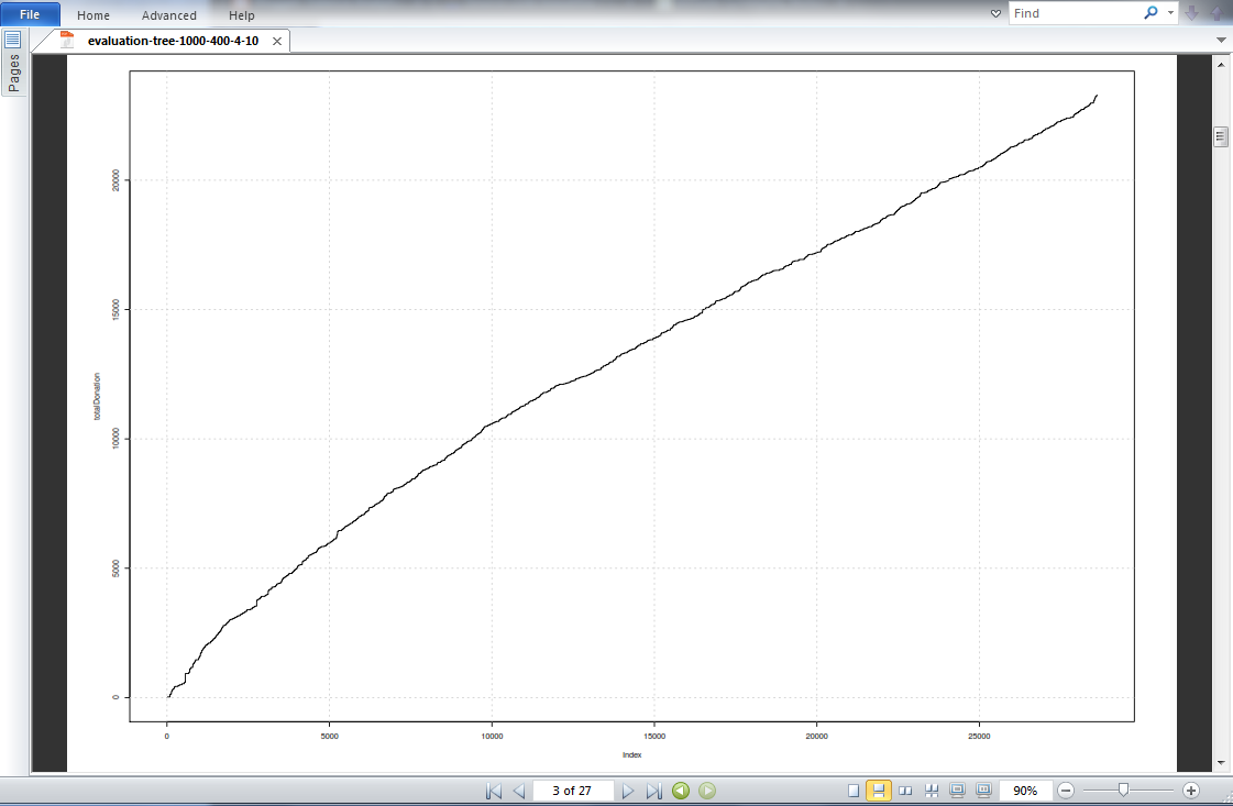
We have a steadily increasing cumulative donation plot, indicating that the tree model did an average job in predicting high donations. The actual donations were indexed by the highest predicted donations so actual high donations should have been plotted first on the x-axis, leading to a sharp increase in the y value at the beginning of the plot.

CSV Output

In our CSV output we saved the "allTotalDonation" and "fnlTotalDonation". The CSV file should be named "evaluation-TotalDonation-1000-400-4-10.csv". Using read.csv() to read in the file, we print out the first fifteen rows of the results. The first column is the index, followed by nine columns of "run.x" loop number, and the average cumulative donation for all nine runs.

CSV Output Code:

1 2 3 4 5 6 7 8 9 10 11 12 13 14 15 16 17 18 19 20 21 22 23 24 25 26 27

> ## 3. interpret results #### > results <- read.csv(paste("evaluation-TotalDonation-", strParameters, ".csv", sep="")) > results[1:15,] X run.1 run.2 run.3 run.4 run.5 run.6 run.7 run.8 run.9 Average 1 1 0 0 0 0 0 0 0 0 0 0.000000 2 2 0 0 10 0 0 0 0 0 0 1.111111 3 3 0 0 10 0 0 0 0 0 0 1.111111 4 4 0 0 10 0 0 0 0 0 0 1.111111 5 5 0 0 10 0 0 0 0 0 50 6.666667 6 6 0 0 10 0 0 0 0 0 50 6.666667 7 7 0 0 10 0 0 0 0 0 50 6.666667 8 8 0 0 10 0 0 0 0 0 50 6.666667 9 9 0 0 10 0 0 0 0 0 50 6.666667 10 10 0 13 10 0 0 0 0 0 50 8.111111 11 11 0 13 10 0 0 0 0 0 50 8.111111 12 12 0 13 10 0 0 0 0 0 50 8.111111 13 13 0 13 10 0 0 0 0 0 50 8.111111 14 14 0 13 10 0 0 0 0 0 50 8.111111 15 15 0 13 27 0 0 0 0 0 50 10.000000 > tail(results) X run.1 run.2 run.3 run.4 run.5 run.6 run.7 run.8 run.9 Average 28619 28619 23264.82 23762.08 22536.67 23885.04 23082.46 21699.42 22479 22477.25 23217.17 22933.77 28620 28620 23284.82 23762.08 22536.67 23885.04 23082.46 21699.42 22479 22477.25 23217.17 22935.99 28621 28621 23284.82 23762.08 22536.67 23885.04 23082.46 21699.42 22479 22477.25 23217.17 22935.99 28622 28622 23284.82 23762.08 22536.67 23885.04 23082.46 21699.42 22504 22477.25 23217.17 22938.77 28623 28623 23284.82 23762.08 22536.67 23885.04 23082.46 21699.42 22504 22477.25 23247.17 22942.10 28624 28624 23284.82 23762.08 22536.67 23885.04 23082.46 21699.42 22504 22477.25 23247.17 22942.10

Next we print out the last six rows with tail(), which displays the cumulative results of each run and the average cumulative donation (not including cost). The average total cumulative donation summed to $22,942.10. Among the runs, ranged from $21,699.42 for run six to $23,885.02 for run four.

Again, this is turning into a lengthy post. After running the loop for one "strParameters" set, we have the predicted donation data. Being optimization, later we will run different "strParameters" to determine which set of models can predict the highest donation return. The next post will explore the donation results data with graphs, in preparation for selecting the best set of decision trees. Stay tuned for more posts!


Thanks for reading,

Wayne
@beyondvalence
LinkedIn

More:
1. KDD Cup: Profit Optimization in R Part 1: Exploring Data
2. KDD Cup: Profit Optimization in R Part 2: Decision Trees
3. KDD Cup: Profit Optimization in R Part 3: Visualizing Results
4. KDD Cup: Profit Optimization in R Part 4: Selecting Trees
5. KDD Cup: Profit Optimization in R Part 5: Evaluation

Predictive Modeling: Decision Trees and Recursive Partitioning in R

A Decision Tree

Hello Readers,


Sometimes we encounter situations where we would like to know the outcome or result of an event given a few factors or variables. In other words, we would like to predict the result. R allows us to create models given the available information to predict what we want to know.

This post will discuss a predictive analysis method, decision trees- a type of non-parametric modeling.


Open R and let us get started!

The Question and the Data

Before approaching the first steps in predictive analysis, keep in mind the result has to answer the question, and the results depends on the analysis we conduct. By initially asking the right question about the data, we can derive a valid answer from the subsequent analysis. Knowing the data, and knowing what we want to discover about the data is an important first step before beginning analysis. So let us look at the dataset.

We will be using the iris dataset already in R. Go ahead open R and call str() on iris to get an idea of the variables in the data.frame. The output is shown below.

str(iris)

Iris is composed of 150 observations with 5 variables which describe the various attributes of the iris plant species. We can plot a few variables by Species to get an idea of the correlation.

Iris Measures Plot

Immediately we can consider whether the first four variables can accurately predict the Species variable. Can we tell which species of iris a particular plant belongs to with some sepal and petal measurements? Let us find out.

Creating The Tree

Start by importing the party package to use decision trees with library(party). Next we will create an index with sample() to separate the data into 70% training data and 30% test data (the seed is 1234 to reproduce the pseudo-random sampling). 

Training and Test Data

Str() the d.train data to verify, and we see that there are 112 observations in d.train, out of the 150 in the original, which is what we wanted (a little over 70%, but it is random).

Next we designate the predictor variables as Sepal.Length, Sepal.Width, Petal.Length, Petal.Width, and the response variable as Species. Then ctree() function creates a binarytree object, and we store it as iris.tree. To see how the iris.tree model compares to the actual species, check it a table:

Iris Tree Formula and Table

We see that all of the setosa species were classified, but versicolor and virginica had 1 and 3 off, respectively- not too shabby. The plot of the iris decision tree is shown below. The petal length was the first chance node, which branched to petal width, then petal length again, creating 4 groups.

Iris Decision Tree

And now that we have 'trained' the data to create the tree classifier, we can predict the the iris species in the d.test data using the predict() function.

Predictions on Iris Test Data

We observe that the setosa and versicolor were predicted well but again, we see that the model missed 2 observations as versicolor when they were in fact, virginica.

Creating Another Tree: Recursive Partitioning

R has several decision tree packages and we will use the rpart package for the next tree. Use library(rpart) to load rpart, and also load the mboost package as well for the bodyfat dataset. Call the str() function on the bodyfat dataset.

Bodyfat Dataset

We will concentrate on predicting the DEXfat levels with the other variables. Again, we will create a separate test and training data sets, so create an index and then use it to create the data sets.

Training and Test Data Sets

Use the age, waistcirc, hipcirc, elbowbreath, and kneebreadth as the predictor variables for DEXfat. In the rpart() function, control the  size of the node to split in the tree by declaring a node to have at least 10 observations.

Bodyfat Tree and Attributes

The bodyfat_rpart is a list containing all the attributes of the decision tree. Next, print the complexity parameter by printing the $cptable in the list. If a split does not decrease the overall lack of fit by a factor of cp, then the split will not occur. The default method uses anova splitting, so the R-squared must increase by cp each step.

Complexity Parameter Table

Next, we can print the tree as shown below. As you can see, it was split 7 times, first by wasitcirc, then by hipcirc and waistcirc and so on.

Bodyfat Tree

To visualize the tree, we use the plot() function, and add the text labels using text() like below:

Plot(), Text(), and the Bodyfat Tree

After which, we can select the tree with the minimum prediction error, from the cptable. The code is illustrated below, where the index of the minimum value of xerror in the cptable is assigned to opt and the respective CP value is passed as the cp value in the prune() function. That yields a tree with a specified prediction error:

Pruning a Tree

Again, we can visualize the newly pruned tree. Notice any differences between the previous tree and the pruned tree?

The Pruned Tree

Yes, the pruned tree does not have the node split from the 4th leaf from the left, instead it ends in the leaf. The xerror from the cp table for that split was greater than the xerror of the previous # 6 split so the pruned tree only has branches up to the lowest prediction error.

Checking the Predictions

Lastly, we will check how the pruned tree predicts DEXfat in the test data set after being fitted to the training data set. Use the predict() function to predict the DEXfat in the b.test data set, and plot the observed vs the predicted to see how close the values are.

DEXfat Prediction and Plot Code

After drawing the perfect prediction line y=x, with abline(), we can see how the predicted values compare with the observed. Note that the values fall generally along the line. The values above the line indicate an over prediction of the values, and those below the line are under predicted.

Predictions vs Observed DEXfat Values

Also, we see that the predicted values come in single values for a ranged of observed values- the values increase by fixed amounts. That is due to the tree classification giving the same predicted value for a set of predictor variables. The observations each leaf will have the same predicted value.

As you can see, decision trees are useful for non-parametric prediction modeling. However, decision trees can over fit the data, so caution must be used, and tree pruning with a predefined acceptable prediction error must be considered for a robust analysis.


Stay tuned for more on prediction modeling and other statistical topics in R!


Thanks for reading,


Wayne
@beyondvalence