Handling Large Data with SQL Server

Hello Readers,

Big Data is all the rage these days. On this blog we have mainly used R as our analysis program of choice (sorry Python) to examine, model, and predict on the data. R is optimal for data with hundred thousands of rows or less, and dealing with larger data sets with millions of rows or more usually slows R down to a crawl. (Remember the neural network post?) Another deciding factor on computation speed is your computer setup. 

Because there are millions of rows in big data sets, we need only sample a few hundred thousand of them into R. But where will we store the millions of rows prior to sampling? Easy, into a data warehouse made for million plus row data sets, a SQL Server database. 

We have not dealt with hundreds of millions or billions of rows, so resist the urge to mention the Hadoop distributed file system. Or should I say not yet? Anyways, here we will load million plus row U.S. Census data sets in preparation for R sampling.

Getting Census Data

Specifically we concentrate on two data sets, U.S. Census American Community Survey 2011, where we can find nationwide population and housing data. You can download the data via ftp here, or choose 2011 ACS 1-year PUMS from the ACS site. The ACS encompasses social, economic, demographic, and housing data. A screenshot of the page is shown below:

Figure 1. American Community Survey (Census) Webpage

After clicking the red highlighted link, 2011 ACS 1-year PUMS, we choose from CSV or SAS file format. Take your pick, I chose CSV for importing into SQL Server.

Figure 2. Choose File Format - CSV

Next, the site gives us choices whether to download the entire dataset for the U.S. or individual states. Of course, download both the Population and Housing data for the entire U.S. Be warned, these two files take up nearly 1 GB of hard drive space, so be patient! Download accelerator anyone?

Figure 3. Download Population and Housing Data Files

After we have the zip files downloaded, unzip them. Note that the housing data 'ss11hus*' and population data 'ss11pus*' have parts a and b.

Figure 4. Unzipped Files

You can also find the helpful README file for the data at the ACS site as well.

Importing into SQL Server

Now for the crucial part, where we import the data into a database system, SQL Server, instead of reading the CSV files into R directly. After connecting to your server, select which database where you would import the CSV files. Right-click and under Tasks, > choose Import Files.

Figure 5. Import Files Option

Next we specify the data source. The CSV files are not Excel or Access files, rather they are a Flat File Source. So select the appropriate option, and select a CSV file from the unzipped file lcoation. On the left you can see a Columns view option under General. You can preview the file contents prior to importing it.

Figure 6. Select Flat File Source

Figure 7 shows the Columns for our preview, so we can ensure the proper headers and values are read by the SQL Server Wizard.

Figure 7. Column Previews

Even though we right-clicked a certain database, SQL Server still asks us in which database we want to import the data. You can change your mind, if you clicked wrong earlier, so take your pick.

Figure 8. Table Destination

Here we encounter the Source Table Option window. We can alter the schema and name of table with Edit Mapping at the bottom. The current schema and name are set as 'dbo' and 'ss11pusa', respectively. If you want to use a different schema than the default, now is the time to impose the change.

Figure 9. Select Source Tables

SQL Server gives us a last overview option before we start the importing process. Ready? Click Finish.

Figure 10. Last Check

And here we go! Look at the Import Wizard chug along as it imports over a million rows!

Figure 11. Import Progressing

When the process is finished, we are rewarded with... a new table lots of rows. Take a look below. 1.6 million? Not bad. Now you just have to import the remaining 3 for a complete set!

Figure 12. Execution Successful

Remember to refresh the Server instance for it to reflect the new table changes. Now you can query away in a new query window to explore the data, or you can keep the Server on and jump into R to establish a database connection using ODBC (open database connectivity).

Figure 13. Locating Imported Table

I thought this post made up for the previous few posts' lack of pictures. Was the compensation count this time sufficient (13)? Here we learned how import a large data set, separated into 4 tables, into a database management system, SQL Server. The next post will feature the next step in accessing Big Data in R, the database connection. There we shall use SQL Server as a data warehouse and R as the analytics tool. Stay tuned.

Thanks for reading,

Wayne
@beyondvalence
LinkedIn

Python: Converting CSV to XML and JSON

Hello Readers,


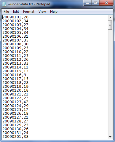
Today we will convert the common CSV (comma separated values) format into XML (extensible markup lanuage) and JSON (javascript object notation) formats in Python. The CSV file we will use was obtained from data scraping the weather underground website.

CSV Data

The CSV data has two elements in each row separated by a comma:
1. The date as 8 characters- 4 year, 2 month, 2 day
2. Temperature in Fahrenheit

CSV To XML

The XML format exists as self-defined tags, beginning with a XML declaration, specifying the XML version "1.0". There is a root element of <weather_data>, and a child element of <observation>, which also has a child element (sub-element) of <date> and <max_temperature>. The root and child elements make up the tree structure, and note that tags need to be closed as well.

XML Tree

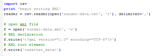
To read the CSV file, we use the csv.reader() method, and set the delimiter to a comma. Then we create the XML file to which we will write the output, and write the XML heading and the root element.

Reading CSV and Writing XML

Now we iterate through the child elements of observations consisting of the date and maximum temperature. Recall that the date is in the first index and the temperature is in the second, with python index starting at 0. Remember to close the open tags afterwards, and close the XML document.

Observation Element and Closing Tags

We can see the results by opening the XML file, and opening it in a web browser, such as Google Chrome:

XML Output

Note how the root and child elements have arrows which we can minimize, and each observation is separate. Our XML formatting looks correct through Chrome. Although the output takes up more room than a CSV file, it is much more readable.

CSV To JSON

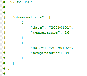
Javascript Object Notation is another format widely used to store and transfer data. It is quite different from XML, because it uses curly braces "{ }" for objects and brackets "[ ]" for arrays, instead of <tags> separating elements. The basic JSON format applied to our weather data is shown below. 

JSON Format

Even though we will not use the json module, I show it so you know it is there. Import the csv module to read our "wunder-data.txt" CSV file again, and write the "observation" object and begin an array with an open bracket. We start a rows_num variable at 0, and count to the max number of iterations (rows in the CSV file).

Import, Read and Write Data

Inside this array, we iterate our observation objects with name/value pairs with date and temperature. Incrementing the rows_num by 1 with each observation, if it reaches 354, we still want to include a comma after the closing curly bracket. But if it reaches 365, then we finish the observations and close the array and observations object.

Iterating Objects

Opening the JSON output in Google Chrome, we see a mess of name/value pairs. Clearly Chrome does not read plain JSON, but there are Chrome Apps available, such as JSONView.

JSON Output

Okay readers, we have covered much ground today with data formats. Both XML and JSON are widely used, knowing both will definitely allow you to utilize varied data sets. Stay tuned for more posts!


Thanks for reading,

Wayne
@beyondvalence