P4.1: Data Modeling in PowerPivot: Relationships

When we wanted to merge two table together, an option would be to use the VLOOKUP function. To analyze the many tables in a data model, VLOOKUP is inefficient and is replaced with relationships, an 'automatic VLOOKUP', which allows us to link entire tables at a time instead of referencing single columns.

As usual, we will be using the Adventure Works companion material (Chapter 4) from the Ferrari book.

Creating the Data Model

Instead of using VLOOKUP multiple times to add columns into the DimProduct table, we will use relationships to merge all three tables together. Opening the PowerPivot window in Diagram View from the workbook we see that the relationships between the tables have already been formed, because PowerPivot detected existing relationships (will be elaborated in further posts.)

Fig. 1: PowerPivot Diagram View

The arrow lines are representations of relationships in Figure 1. The arrow starts at DimProduct, the source table and points to DimProductSubcategory, the target table, and the connection is finished as DimProductSubcategory is linked to the DimProductCategory table. In the measure field towards the bottom half in grid view of the DimProduct table, we can add a calculated field for the number of products, NumOfProducts. 

Fig. 2: Creating NumOfProducts Calculated Field

Now we can create a PivotTable tabulating the number of products for each ProductCategory from the DimProduct table. The ProductCategory is actually the EnglishProductCategoryName field in the DimProductCategory table, two relationships away, connected by the ProductSubcategoryKey and the ProductCategoryKey.

Fig. 3: ProductCategory PivotTable

Data models are much more efficient in performance compared to VLOOKUP, especially when dealing with large data sets for computational power, and in multiple tables for a chain of relationships. Also, the NumOfProduct field calculation is available for any PivotTable using the data model, so we do not have to create a new definition every time.

So a data model is a set a tables connected by relationships, sometimes with calculated fields or columns. Simple yet powerful.

Notes on Relationships

Though these relationships will not help much in your love life, the following details on PowerPivot relationships will make your life easier when creating and understanding data models.

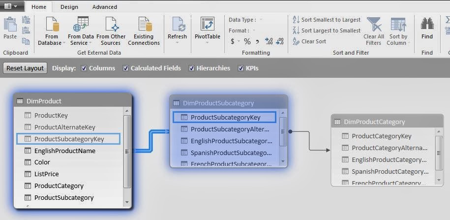
Looking at the Diagram View of the tables and relationships, we focus on the relationship arrow from DimProduct to DimProductSubcategory.

• DimProduct is the source table (the beginning of the relationship)
• DimProductSubcategory is the target table (where the values relate to source table)
• ProductSubcategoryKey column is the Foreign Key in source table (contains values which is searched in target table for related row)
• ProductSubcategoryKey column is the Primary Key in the target table (needs to have unique values in each row)

These are shown highlighted in blue below:

Fig. 4: DimProduct and DimProductSubcategory Relationship

A specific product can only have one subcategory, whereas a subcategory may have many products. That is why the target table (DimProductSubcategory) must have an unique Primary Key (ProductSubcategory) for the products in the DimProduct table. This type of relationship is called "one-to-many", with the target table being "one side", and the source table being the "many side" of the relationship.

We can test the relationship by recreating it. Click the arrow and press Delete. Then in the Design tab, click Create Relationship.

Fig. 5: Creating a Relationship

In the drop-down boxes, we would want to specify the DimProduct and DimProductSubcategory as tables, with the ProductSubcategoryKey as columns from both. However, if we accidentally flip the tables, and confuse the "one-to-many" to "many-to-one" tables, PowerPivot automatically detects the columns in the tables and lets us know it will create the relationship in the opposite direction.

So now you know the inner workings of relationships in data models. Some DAX functions work only when invoked on the correct side of a relationship, so sides do matter. Stay tuned for more on data modeling!


Thanks for reading,

Wayne

P1.1: VLOOKUP and PivotTables in PowerPivot- Excel 2013

This post describes how to add data from other sheets using VLOOKUP, and make a PivotTable in Excel 2013 from the PivotTable workbook in Chapter 1 of the PowerPivot book.

VLOOKUP 

By opening the PivotTable workbook in Excel you can observe the relevant data for the fictional products of the example company, AdventureWorks. Figure 1 shows a segment of the data.

Fig. 1: AdventureWorks Sales data

The SalesManager column (B) was added to the Sales sheet using the VLOOKUP function (Figure 2) from the data in the SalesManagers sheet (Figure 3). 

=VLOOKUP([@ProductCategory], SalesManagers, 2)

The above VLOOKUP function matches the elements of the ProductCategory field of the current (Sales) sheet to first column of the SalesManager sheet, and retrieves the element of the corresponding second column (SalesManager) of the SalesManagers sheet. So, the Sales Manager of a specific product category shown on the SalesManagers sheet will be added to the respective category of product on the Sales sheet.

Fig. 2: VLOOKUP adding Sales Manager column in Sales sheet

Fig. 3: SalesManagers sheet

Although VLOOKUP is useful, it will be difficult and cumbersome if you want to analyze additional variables by adding them one by one. Relationships and Excel data models will be explored in the next post which will allow complete table analysis (not just one column at a time), and multi-table analysis (many columns of many tables).

PivotTables

This information is stored as an Excel table. To make a PivotTable, which allows analysis of many fields, and later can be linked together into a data model, Excel requires PowerPivot to be enabled in Excel 2013, and downloaded and installed for Excel 2010. (Click here on how to enable PowerPivot in Excel versions 2013 or 2010.) When PowerPivot is enabled, you should see the PowerPivot displayed in Excel's ribbon tab at the top right (Figure 4).

Fig. 4: PowerPivot tab in Excel 2013

To add a PivotTable of the AdventureWorks data, you click the Insert tab and then select the PivotTable button on the ribbon. An option window pops up, so you can select what data to analyze, and where to put the new PivotTable, as shown in Figure 5.

Fig. 5: PivotTable options

After you click OK, the blank PivotTable appears (Figure 6), ready for fields to be added to the report.

Fig. 6: Blank PivotTable with Fields on right side

From the right hand side in the PivotTable Fields, you can select the desired items to analyze and drag them to the appropriate quadrant in the bottom right corner, below the PivotTable Fields list. 

To produce a report regarding the total sales from 2005-2008 of categorized products sold under all sales managers, you select the ProductCategory, SalesManager, Year, and SalesAmount fields and drag them to the areas of rows for the first two, columns and values for the last two, as shown below in Figure 7.

Fig. 7: PivotTable with Sales of Products by Sales Managers by Year

There you have your PivotTable.

Thanks for reading,
Wayne