R: Classifying Handwritten Digits (MNIST) using Random Forests

Hello Readers,


The last time we used random forests was to predict iris species from their various characteristics. Here we will revisit random forests and train the data with the famous MNIST handwritten digits data set provided by Yann LeCun. The data can also be found on Kaggle.

We will require the training and test data sets along with the randomForest package in R. Let us get started. (Click here for the post that classifies MNIST data with a neural network.)

Scribbles on Paper

Hand writing is unique to each person, and specifically the numbers we write have unique characteristics (mine are difficult to read). Yet when we read numbers written by other people, we can very quickly decipher which symbols are what digits. 

Since there is increasing demand to automate reading handwritten text, such as ATMs and checks, computers must be able to recognize digits. So how can we accurately and consistently predict numbers from hand written digits? The data set provided by Yann LeCun was originally a subset of the data set from NIST (National Institute of Standards and Technology) sought to tackle this problem. Using various classifier methods LeCun was able to achieve test error rates of below 5% in 10,000 test images.

The data set itself consists of training and test data describing grey-scale images sized 28 by 28 pixels. The columns are the pixel number, ranging from pixel 0 to pixel 783 (786 total pixels), which have elements taking values from 0 to 255. The training set has an additional labels column denoting the actual number the image represents, so this what we desire from the output vector from the test set.

As we can see, the image numbers are in no particular order. The first row is for the number 1, the second for 0, and third for 1 again, and fourth for 4, etc.

MNIST Training Data

Before we create the random forest, I would like to show you the images of the digits themselves. The first 10 digits represented by the first 10 rows of written numbers from the training data are shown below.

Handwritten Numbers

How did we obtain those PNG images? I formed a 28 x 28 pixel matrix from the training data rows and passed it to the writePNG() function from the png library to output numerical images. Since the values range from 0 to 255, we had to normalize them from 0 to 1 by dividing them by 256.

Creating a PNG of First Row

The above code will create a png file for the first row (digit) in the training set. And it will give us this:  , a one. The below code stacks the rows 1 to 5 on top of the rows 6 through 10.

Creating a Stacked PNG for 10 Digits

And the image resulting from the above code we saw already, as the first series of handwritten numbers above.

Random Forests

Now that we know how the image was mapped onto the data set, we can use random forests to train and predict the digits in the test set. With the randomForest package loaded, we can create the random forest:

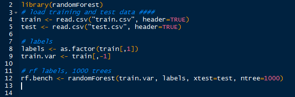Creating RandomForest

After taking out the labels in the training set, we can use train.var, with corresponding training output as labels, and the test data as test. We will use 1,000 trees (bootstrap sampling) to train our random forest. Note that the creation of this random forest will take some time- over an hour on most computers. I left R running overnight to ensure that it would be completed by morning. Timed with proc.time(), it took about 3 hours on my (slow) computer.

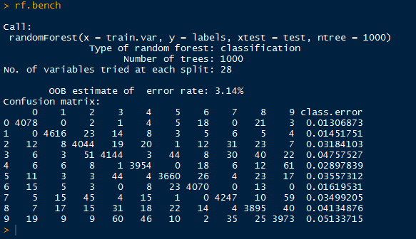RandomForest

Above, we have the default output of the random forest, containing the out-of-bag error rate (3.14%), and a confusion matrix informing us how well the random forest classified the 0-9 labels with the actual labels. We see large numbers down the diagonal, but we should not stop there.

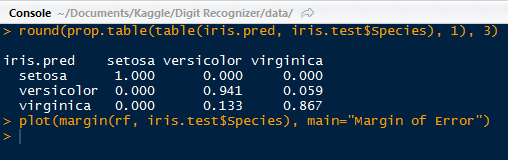
Then we can call plot() on rf.bench to visualize the error rates as the number of trees increase:

plot(rf.bench)

We see that the aggregate OOB errors decrease and approach 0.0315, as in the output. The OOB error rate describes the error of each bootstrapped sampled tree with 2/3rds of the data and uses the "out of bag" remaining 1/3rd, non-sampled data to obtain a classification using that tree. The error from the classification using that particular tree is the OOB error.

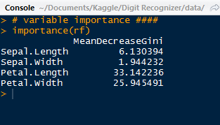
Next we can observe which variables were most important in classifying the correct labels by using the varImpPlot() function.

Important Pixels

We can see the most important pixels from the top down- #378, 350, 461, etc. There is another step where we can rerun the random forest using the most important variables only.

Predicting Digits

Lastly, we need to predict the digits of the test set from our random forest. As always, we use the predict() function. However, since we already specified the test data in our randomForest() function, all we need to do is call the proper elements in the object. By using rf.bench$test$predicted we can view the predicted values. The first 15 are down below:

First 15 Predicted Digits

After using the write() function to write a csv file, we can submit it to Kaggle (assuming you used the Kaggle data) to obtain the score out of 1 for the proportion of test cases our random forest successfully classifies. We did relatively well at 0.96757.

Kaggle Submission

And there we have it, folks! We used random forests to create a classifier for handwritten digits represented by grey-scale values in a pixel matrix. And we successfully were able to classify 96.8% of the test digits. 

Stay tuned for predicting more complex images in later posts!


Thanks for reading,

Wayne
@beyondvalence
LinkedIn

Predictive Modeling: Creating Random Forests in R

Hello Readers,

Welcome back to the blog. This Predictive Modeling Series post will cover the use of Random Forests in R. Before we covered decision trees and now we will progress a step further in using multiple trees.

Click here to read Leo Breiman's paper for random forests.


Load the randomForest library package in R, and let us begin!

Iris Data

We will use the familiar iris data set found in previous posts as well. To remind us what we are working with, call head() on iris. 

Load randomForest and iris data

We are looking at four variables of the flowering iris plant and the fifth variable indicates the species of the flower. Now we can separate the data into a training set for the random forest and a testing set to determine how well the random forest predicts the species variable.

First sample 1 and 2 from the row number of the data set. We set the probability of 1 at 0.7 and 2 at 0.3 so that we get a larger training set. Then we assign the respective subsets of iris to their training and testing sets.

Creating Training and Test Data

Now that we have our data sets, we can perform the random forest analysis.

Random Forest

The Random Forest algorithm was developed by Leo Breiman and Adele Cutler. Random Forests are a combination of tree predictors, such that each tree depends on a random vector sampled from all the trees in the forest. This incorporates the "bagging" concept, or bootstrap aggregating sample variables with replacement. It reduces variance and overfitting. Each tree is a different bootstrap sample from the original data. After the entire ensemble of trees are created, they vote for the most popular class.

With the randomForest package loaded, we can predict the species variable with the other variables in the training data set with 'Species ~ .' as shown below. We are going to create 100 trees and proximity will be true, so the proximity of the rows values will be measured.

iris Random Forest

See that we have results of the random forest above as well. The 'out of bag' estimate is about 4.59%, and we have the confusion matrix below that in the output. A confusion matrix, otherwise known as a contingency table, allows us to visualize the performance of the random forest. The rows in the matrix are the actual values while the columns represent the predicted values.

We observe that only the species setosa has no classification error- all of the 37 setosa flowers were correctly classified. However, the versicolor and virginica flowers had errors of 0.057 and 0.081 respectively. 2 versicolors were classified as virginica and 3 virginicas were classified as versicolor flowers.

Call attributes() on the random forest to see what elements are in the list.

Attributes of iris Random Forest

Visualizing Results

Next we can visualize the error rates with the various number of trees, with a simple plot() function.

plot(rf)

Though the initial errors were higher, as the number of trees increased, the errors slowly dropped somewhat over all. The black line is the OOB "out of bag" error rate for each tree. The proportion of times of the top voted class is not equal to the actual class is the OOB error.

We observe which predictors were more important with the importance() function. As we can see, the most important variable was Petal.Length.

Important Predictors

Using the varImpPlot() function, we can plot the importance of these predictors:

For our most important variables for classification are Petal.Length and Petal.Width, which have a large gap between the last two sepal variables. Below we have the species predictions for the iris test data, obtained by using the prediction() function.

Iris Test Contingency Table

We see again that the setosa species performed relatively better than the versicolor and virginica. With the prop.table() function nested outside of the table() function, we can create a table for the proportions. Versicolor performed second best with 94% correct and virginica with 86%.

Proportion Table with Plot Code

We can go ahead a create a plot of the margin of error. The margin for a particular data point is the proportion of votes for the correct class minus the maximum proportion of votes of the other classes. Generally, a positive margin means correct classification.

Margin of Error Plot

We can see that as the most of the 100 trees were able to classify correctly the species of iris, although the few at the beginning were below 0. They had incorrectly classified the species.

Overall, the random forests method of classification fit the iris data very well, and is a very power method of classifier to use in R. Random forests do not overfit the data, and we can implement as many trees as we would like. It also helps in evaluating the variables and telling us which ones where most important in the model.

Thanks for reading,


Wayne
@beyondvalence