Python and Pandas: Part 2. Movie Ratings

Hello Readers,

Here is Part 2 of the Pandas and Python series, where we examine movie ratings data from University of Minnesota's Movielens recommendation system. The 1 million rows of data are available here as a 'zip' and 'readme' file. We will use Pandas in Python to read, manipulate, and massage the rating data. The sizable data include over 1 million ratings from 6,000 users, concerning 4,000 movies.

As a reference, I am using Python 2.7.8 via IPython 2.1.0. Start IPython and let's jump in.

Loading the Rating Data

After navigating to the proper directory with the three ending in .dat, start IPython with "matplotlib". Immediately import "pylab" and "pandas". While loading the user, rating and movie data files, we create the variable names for each DataFrame. 

For example, the "users" DataFrame has "user_id", "gender", "age", "occupation", and "zip" code for its variables. Preview the first 5 rows by slicing "[:5]".

Code:

1 2 3 4 5 6 7 8 9 10 11 12 13 14 15 16 17 18 19 20 21 22 23 24 25 26 27 28 29 30 31 32 33 34 35 36 37 38 39 40 41 42 43 44 45 46 47 48 49 50 51 52 53 54 55 56 57 58 59 60 61 62 63 64 65

C:\Users\wayne\Documents\python\dataAnalysis\git\ch02>ipython --matplotlib Python 2.7.8 (default, Jun 30 2014, 16:03:49) [MSC v.1500 32 bit (Intel)] Type "copyright", "credits" or "license" for more information. IPython 2.1.0 -- An enhanced Interactive Python. ? -> Introduction and overview of IPython's features. %quickref -> Quick reference. help -> Python's own help system. object? -> Details about 'object', use 'object??' for extra details. Using matplotlib backend: Qt4Agg In [1]: import pylab In [2]: import pandas as pd In [3]: unames = ['user_id','gender','age','occupation','zip'] In [4]: users = pd.read_table('movielens/users.dat',sep='::',header=None, ...: names=unames) In [5]: users[:5] Out[5]: user_id gender age occupation zip 0 1 F 1 10 48067 1 2 M 56 16 70072 2 3 M 25 15 55117 3 4 M 45 7 02460 4 5 M 25 20 55455 In [16]: rnames = ['user_id','movie_id','rating','timestamp'] In [17]: ratings = pd.read_table('movielens/ratings.dat',sep='::',header=None,names=rnames) In [18]: ratings[:5] Out[18]: user_id movie_id rating timestamp 0 1 1193 5 978300760 1 1 661 3 978302109 2 1 914 3 978301968 3 1 3408 4 978300275 4 1 2355 5 978824291 In [19]: mnames = ['movie_id','title','genres'] In [20]: movies = pd.read_table('movielens/movies.dat',sep='::',header=None,names=mnames) In [21]: movies[:5] Out[21]: movie_id title genres 0 1 Toy Story (1995) Animation|Children's|Comedy 1 2 Jumanji (1995) Adventure|Children's|Fantasy 2 3 Grumpier Old Men (1995) Comedy|Romance 3 4 Waiting to Exhale (1995) Comedy|Drama 4 5 Father of the Bride Part II (1995) Comedy In [22]: ratings Out[22]: <class 'pandas.core.frame.DataFrame'> Int64Index: 1000209 entries, 0 to 1000208 Data columns (total 4 columns): user_id 1000209 non-null values movie_id 1000209 non-null values rating 1000209 non-null values timestamp 1000209 non-null values dtypes: int64(4)

Looking at the "ratings" DataFrame specifically, we find that it has 1,000,209 entries (rows), with 4 columns- "user_id", "movie_id", "rating", and "timestamp". We see that the ratings are integers up to 5. The common variables among the 3 DataFrames are "user_id" and "movie_id".

Merging DataFrames

Working with three data from three separate DataFrames will hamper our efficiency in querying rows we require for analysis. The files were normalized for size efficiency for downloading, and now since we have them on our hard drive, we can go ahead and merge them together (de-normalize). 

Once we merge the DataFrames, there will be redundant elements, as user information will be repeated for various movies they rated, and movie information will be repeated as well since movies have multiple users rating them. That is why the file will be larger in size (think megabytes vs kilobytes). For storage purposes, a normalized format is more optimal, whereas for fast read/write times, de-normalized tables are more efficient.

From pandas, use the ".merge()" method twice to merge all three DataFrames together. The method will merge by similar column names, which is why we named them "user_id", "movie_id". 

Code:

1 2 3 4 5 6 7 8 9 10 11 12 13 14 15 16 17 18 19 20 21 22 23 24 25 26 27 28 29 30 31 32

In [23]: data = pd.merge(pd.merge(ratings,users),movies) In [24]: data Out[24]: <class 'pandas.core.frame.DataFrame'> Int64Index: 1000209 entries, 0 to 1000208 Data columns (total 10 columns): user_id 1000209 non-null values movie_id 1000209 non-null values rating 1000209 non-null values timestamp 1000209 non-null values gender 1000209 non-null values age 1000209 non-null values occupation 1000209 non-null values zip 1000209 non-null values title 1000209 non-null values genres 1000209 non-null values dtypes: int64(6), object(4) In [25]: data.ix[0] Out[25]: user_id 1 movie_id 1193 rating 5 timestamp 978300760 gender F age 1 occupation 10 zip 48067 title One Flew Over the Cuckoo's Nest (1975) genres Drama Name: 0, dtype: object

Now the complete table has 1,000,209 rows with 10 variable columns. Taking the first row index with ".ix[0]", we can examine the merge results within the first row. This female gave the movie "One Flew Over the Cuckoo's Nest" the highest 5 star rating. And looking at her age, 1, we only know that she is less than 18 years of age. Note that the occupation categories are explained in the included README file. (Go ahead, read it).

Pivot Table

Since there are 10 variables, we can massage the data into showing us some patterns between the variables. Not only can we see the average ratings for each movie, we can stratify them by gender. We accomplish this with ".pivot_table()", while specifying the value we want stratified, the variables we want to see in the rows and columns, and how we want to values to be presented (mean).

Taking the first 8 movies, and observe that they are ordered alphabetically by symbol/punctuation, numbers, capitalized letters, and lowercase letters. We can see the average ratings for the movies by gender.

Code:

1 2 3 4 5 6 7 8 9 10 11 12 13 14

In [26]: mean_ratings = data.pivot_table('rating',rows='title',cols='gender',aggfunc='mean') In [27]: mean_ratings[:8] Out[27]: gender F M title $1,000,000 Duck (1971) 3.375000 2.761905 'Night Mother (1986) 3.388889 3.352941 'Til There Was You (1997) 2.675676 2.733333 'burbs, The (1989) 2.793478 2.962085 ...And Justice for All (1979) 3.828571 3.689024 1-900 (1994) 2.000000 3.000000 10 Things I Hate About You (1999) 3.646552 3.311966 101 Dalmatians (1961) 3.791444 3.500000

For the cartoon, 101 Dalmations released in 1961, the average female rating was ~3.79, while the average male rating was slightly lower at 3.50. Sometimes the average rating would be close, and others one gender would rate a movie more favorably than the other gender.

Movie Rating Subsetting and Sorting

Here we aim to work with a robust set of movies with 250 or more ratings by subsetting the data. First we create an index in active_titles of movies grouped by their title using ".groupby('title').size()" or their count. Then using the ratings_by_title, we select only those with 250 or more ratings through the ".index[]" into active_titles.

From the gender stratified mean_ratings created above, we can subset those movies titles with 250 or more ratings, with ".ix[]" for index. Now the DataFrame is reduced to 1,216 movies, from 6,000.

Code:

1 2 3 4 5 6 7 8 9 10 11 12 13 14 15 16 17 18 19 20 21 22 23 24 25 26 27 28 29 30 31 32 33 34 35 36 37 38 39 40 41 42 43 44 45 46 47 48 49

In [9]: ratings_by_title = data.groupby('title').size() In [10]: ratings_by_title[:10] Out[10]: title $1,000,000 Duck (1971) 37 'Night Mother (1986) 70 'Til There Was You (1997) 52 'burbs, The (1989) 303 ...And Justice for All (1979) 199 1-900 (1994) 2 10 Things I Hate About You (1999) 700 101 Dalmatians (1961) 565 101 Dalmatians (1996) 364 12 Angry Men (1957) 616 dtype: int64 In [11]: active_titles = ratings_by_title.index[ratings_by_title >= 250] In [12]: active_titles Out[12]: Index(['burbs, The (1989), 10 Things I Hate About You (1999), 101 Dalmatians (1961), ..., Young Sherlock Holmes (1985), Zero Effect (1998), eXistenZ (1999)], dtype=object) In [13]: mean_ratings = mean_ratings.ix[active_titles] In [14]: mean_ratings Out[14]: <class 'pandas.core.frame.DataFrame'> Index: 1216 entries, 'burbs, The (1989) to eXistenZ (1999) Data columns (total 2 columns): F 1216 non-null values M 1216 non-null values dtypes: float64(2) In [15]: top_female_ratings = mean_ratings.sort_index(by='F',ascending=False) In [16]: top_female_ratings[:10] Out[16]: gender F M title Close Shave, A (1995) 4.644444 4.473795 Wrong Trousers, The (1993) 4.588235 4.478261 Sunset Blvd. (a.k.a. Sunset Boulevard) (1950) 4.572650 4.464589 Wallace & Gromit: The Best of Aardman Animation (1996) 4.563107 4.385075 Schindler's List (1993) 4.562602 4.491415 Shawshank Redemption, The (1994) 4.539075 4.560625 Grand Day Out, A (1992) 4.537879 4.293255 To Kill a Mockingbird (1962) 4.536667 4.372611 Creature Comforts (1990) 4.513889 4.272277 Usual Suspects, The (1995) 4.513317 4.518248

From this refined data, we can reorder and display the top rated titles by females with ".sort_index()". The top female averaged rated title goes to 'A Close Shave', with 'The Wrong Trousers' coming in second. While the average male ratings were not ordered, they are similar in range, due to the quality of the movies. So, users enjoying a movie would be more inclined to rate a movie, thus this subset of movies with 250+ ratings is slightly more biased than the original total data.

Measuring Rating Disagreement

However females and males did not rate movies similarly. We can create a new variable, 'diff', for rating difference of males - females. Then we can sort the mean_ratings with the largest difference first. The biggest disparity in rating where female movie ratings measured higher than males belonged to 'Dirty Dancing', 'Jumpin' Jack Flash', and 'Grease'.

Code:

1 2 3 4 5 6 7 8 9 10 11 12 13 14 15 16 17 18 19 20 21 22 23 24 25 26 27 28 29 30 31 32 33 34 35 36 37 38 39 40 41 42 43 44 45 46 47 48 49 50 51 52 53 54 55 56 57 58 59

## measuring rating disagreement In [17]: mean_ratings['diff'] = mean_ratings['M'] - mean_ratings['F'] In [19]: sorted_by_diff = mean_ratings.sort_index(by='diff') In [20]: sorted_by_diff[:10] Out[20]: gender F M diff title Dirty Dancing (1987) 3.790378 2.959596 -0.830782 Jumpin' Jack Flash (1986) 3.254717 2.578358 -0.676359 Grease (1978) 3.975265 3.367041 -0.608224 Little Women (1994) 3.870588 3.321739 -0.548849 Steel Magnolias (1989) 3.901734 3.365957 -0.535777 Anastasia (1997) 3.800000 3.281609 -0.518391 Rocky Horror Picture Show, The (1975) 3.673016 3.160131 -0.512885 Color Purple, The (1985) 4.158192 3.659341 -0.498851 Age of Innocence, The (1993) 3.827068 3.339506 -0.487561 Free Willy (1993) 2.921348 2.438776 -0.482573 In [21]: sorted_by_diff[::-1][:15] Out[21]: gender F M diff title Good, The Bad and The Ugly, The (1966) 3.494949 4.221300 0.726351 Kentucky Fried Movie, The (1977) 2.878788 3.555147 0.676359 Dumb & Dumber (1994) 2.697987 3.336595 0.638608 Longest Day, The (1962) 3.411765 4.031447 0.619682 Cable Guy, The (1996) 2.250000 2.863787 0.613787 Evil Dead II (Dead By Dawn) (1987) 3.297297 3.909283 0.611985 Hidden, The (1987) 3.137931 3.745098 0.607167 Rocky III (1982) 2.361702 2.943503 0.581801 Caddyshack (1980) 3.396135 3.969737 0.573602 For a Few Dollars More (1965) 3.409091 3.953795 0.544704 Porky's (1981) 2.296875 2.836364 0.539489 Animal House (1978) 3.628906 4.167192 0.538286 Exorcist, The (1973) 3.537634 4.067239 0.529605 Fright Night (1985) 2.973684 3.500000 0.526316 Barb Wire (1996) 1.585366 2.100386 0.515020 In [33]: rating_std_by_title = data.groupby('title')['rating'].std() In [34]: rating_std_by_title = rating_std_by_title.ix[active_titles] In [35]: rating_std_by_title.order(ascending=False)[:10] Out[35]: title Dumb & Dumber (1994) 1.321333 Blair Witch Project, The (1999) 1.316368 Natural Born Killers (1994) 1.307198 Tank Girl (1995) 1.277695 Rocky Horror Picture Show, The (1975) 1.260177 Eyes Wide Shut (1999) 1.259624 Evita (1996) 1.253631 Billy Madison (1995) 1.249970 Fear and Loathing in Las Vegas (1998) 1.246408 Bicentennial Man (1999) 1.245533 Name: rating, dtype: float64

Conversely, if we flipped the order around, where the male ratings were higher than female ratings, the differential pointed to 'The Good, The Bad and the Ugly', 'The Kentucky Fried Movie', and 'Dumb & Dumber'. Both sets of films, while good, cater stereo-typically to different genders.

Another way to measure the differential is through the spread, otherwise known as the standard deviation. Among all movies and users, 'Dumb & Dumber' took the top prize with the highest standard deviation of 1.321. Therefore, the ratings users assigned to 'Dumb & Dumber' differed more among each other than for other movies, although 'The Blair Witch Project' came in a close second at 1.316

Average User Age by Movie

Grouping by movie, we can find the average age of the user who rates the movies. We also use active_titles to subset those movies with a large number of ratings. The movies with the youngest users rating them are: 'Can't Hardly Wait', 'Friday', and 'Empire Records', all just over 21. Note the year of the movies are more recent in the 1990s or 2000.

On the older end, the highest average age rated movies turned out to be: 'Hud', 'Klute', and 'Around the World in 80 Days'. Again, note the movie dates as they are in the 1960s, 1970s, and 1980s, more resonant with more esteemed users who have seen the movies when they were younger.

Code:

1 2 3 4 5 6 7 8 9 10 11 12 13 14 15 16 17 18 19 20 21 22 23 24 25 26 27 28 29 30 31 32

In [37]: avg_age = data.groupby('title')['age'].mean() In [45]: avg_age = avg_age.ix[active_titles] In [47]: avg_age.order(ascending=True)[:10] Out[47]: title Can't Hardly Wait (1998) 21.284314 Friday (1995) 21.768025 Empire Records (1995) 21.940959 Billy Madison (1995) 22.253521 Mallrats (1995) 22.432373 Road Trip (2000) 22.584726 Scream 3 (2000) 22.818024 Teenage Mutant Ninja Turtles II: The Secret of the Ooze (1991) 23.107570 Skulls, The (2000) 23.463576 Tommy Boy (1995) 23.585366 Name: age, dtype: float64 In [48]: avg_age.order(ascending=False)[:10] Out[48]: title Hud (1963) 41.971326 Klute (1971) 40.817881 Around the World in 80 Days (1956) 40.732342 Tender Mercies (1983) 40.196970 Breaker Morant (1980) 39.655556 Cat Ballou (1965) 39.575000 Atlantic City (1980) 39.483553 Mister Roberts (1955) 39.323040 Taking of Pelham One Two Three, The (1974) 39.217391 In the Heat of the Night (1967) 38.681034

Take heed though, of the age group less than 18. It is numerated with 1. So taking the average age is somewhat misleading, as those less than one skew the mean more than their actual age would. I assume that one year-olds would not be rating movies. We will have to correct this issue later.


Well, congratulations on reaching the end of this picture-less post! Here we used pandas in Python to create and merge DataFrames, and created more specific-use DataFrames through subsetting, and viewing the various orders through sorting. I hope you have an idea of the versatility of Python for data analysis with pandas by reading this series! Stay tuned for more posts!



Thanks for reading,

Wayne
@beyondvalence
LinkedIn


Python and Pandas Series:
1. Python and Pandas: Part 1: bit.ly and Time Zones
2. Python and Pandas: Part 2. Movie Ratings
3. Python and Pandas: Part 3. Baby Names, 1880-2010
4. Python and Pandas: Part 4. More Baby Names
.

P3.2: Beginning DAX 2

And we are back again for more DAX! This post is a continuation in the understanding DAX series (link to P3.1.) Here we will gain a deeper understanding of calculated columns and fields (introduced in P2.2) from a DAX perspective.

Understanding Calculated Columns & Fields

Calculated columns and calculated fields are actually quite different despite initial similarities. Here we will explore the differences of columns of fields, while gaining DAX concepts and syntax.

Calculated Columns

Before in P2.2, we touched upon the notion of creating a calculated column and a calculated field. By clicking the Add Column button on the Design tab, we can create a calculated column in PowerPivot. It is versatile in PivotTables; also the DAX expression for the column applies to the current row of the table. When we reference a column, it returns the value of that particular column in that specific row.

Fig. 1: Add Column Button

Note:
There are DAX functions which aggregate the values of a column for a whole table. To evaluate a subset of rows, we use DAX to specify a range of rows or a single value from another row and operate on that subset table. Essentially we can restrict rows and apply filters so the desired rows are selected for computation.

Calculated Fields

Now for something a little different. While calculated fields use the same DAX syntax as calculated columns, calculated fields evaluate the expression at the context of the cell of the PivotTable, not at the row level of the PowerPivot table like a calculated column.

Fig. 2: Calculated Fields Button

Which is why we arrived at a wrong result when we tried to calculate the gross margin as a percentage of the sales as a calculated column. In fact, PowerPivot calculated the gross margin percentage for each row using that method. What we wanted was to divide the gross margin by the sales within the context (column and row designation) of the PivotTable; we did not want each percentage in each row added, we required the gross margin percentage of the total (in say, Year 2006.)

So if we used the regular formula to calculate a field, we could get the following error:

Fig. 3: Calculated Field Error Using the Same DAX Expression as Calculating a Column

That is because the GrossMargin column has a different value in each row, and we would rather see the aggregate of the GrossMargin divided by the aggregate SalesAmount for each cell context in the PivotTable.

The correct method was to type in the sum of each:
=SUM(Sales[GrossMargin]) / SUM(Sales[SalesAmount])
and then divide them, as shown in Figure 4.

Fig. 4: Using the SUM for the Correct Calculated GrossMarginPct Field (See: No Errors!)

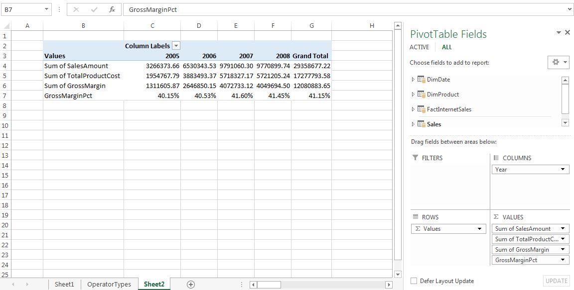
By using this approach, in the PivotTable, the column and row would have the labels as the context for the cells involved. So when it goes to take the SUM of the GrossMargin and the SUM of the SalesAmount, this specific PivotTable takes the SUM for a certain Year context, and summing values in the DAX expression, say for 2007. The PivotTable with GrossMarginPct added is shown below.

Fig. 5: PivotTable with GrossMarginPct

When to Use Calculated Columns and Measures (Fields)

So when do we use a calculated column and in other cases, a calculated field (or measure)? (When do we get to eat Jell-O?) In most situations, it would depend on the computation of choice. For example, there are several situations to use calculated columns:

• When we want to evaluate an expression which is confined to the current row,
• The results will be displayed in the columns or rows of the PivotTable, and not the values,
• Or when we categorize text or numbers (categorical variables)

Situations where we would use calculated fields occur when we would like to display the results in the PivotTable Values section. Each cell in the Values section will change based on the context of the rows and columns in the PivotTable selections. If we changed the rows in Figure 5 to include the ModelName, then the calculationed field would reflect the change, and show the GrossMarginPct stratified by ModelName (Figure 6).

Fig. 6: PivotTable with ModelName Stratifying the Calculated Field

Cross-Referencing

We can use calculated columns in our DAX expressions when creating calculated fields. Also, the reverse can be done as well. However counter-intuitive, a calculated column can reference calculated fields, and this confines the calculated field to the context of the current row. Therefore, the calculated field transforms into a calculated column, and will not be influenced by user changes in context on the PivotTable.


Here we have explored the similarities and (for the most part) differences between calculated columns and fields through DAX. Understanding these concepts are important in becoming proficient at DAX, as well being able to manipulate data efficiently.


Thanks for reading,

Wayne

P2.3: Computing Complex Aggregations in PowerPivot: Distinct Count & Refreshing the Data Model

This post will describe how to calculate a complex aggregation such as a distinct count of products in PowerPivot. We will be using the data model created in the previous post, from the companion material of the Ferrari PowerPivot book.

Computing Distinct Count

Calculated fields have an useful feature that enables us to compute complex aggregations. In the last post we calculated the gross margin and also the gross percentage of sales using calculated column and field. Today we would like to determine the number of products in each Color.

Let us begin by creating a simple PivotTable showing the SalesAmount by Color of products.

Fig. 1: Sum of SalesAmount by Color of Product

We want to count the number of products, not the number sold under each Color; whether a particular product sold 8,000 units or only 1 unit, the count would only be 1 for that same product (hence distinct count.)

If we add the ProductKey under the DimProduct table to the PivotTable, we can see that the result is not what we were looking for.

Fig. 2: PivotTable with Sum of ProductKey

From the numbers and the column header, the column is displaying the sum of the product keys. It is logical that Excel took the sum because the values are integers. However we want the sum of the number of unique product keys. We can change the method Excel aggregates the data, by changing the settings of ProductKey in the Values area. Click the drop-down arrow and select the Value Field Settings button.

Fig. 3: Value Field Settings Button

In the Value Field Settings window, we can select an attractive option, which also happens to be called Distinct Count. Note that the Custom Name of the column changes to "Distinct Count of ProductKey".

Fig. 4: Value Field Settings- Distinct Count Option

Now let us observe the new PivotTable showing the proper distinct count. The two red arrows point to rows with counted products but no sales. If we want to count products responsible for sales, we should only count those products that were actually sold. 

Fig. 5: PivotTable with Corrected Distinct Count

The correct field to display in the PivotTable is the ProductKey under the FactInternetSales table, because the table has only product keys of products that were sold. This highlights how easily we could choose the wrong field to aggregate, especially for the computation of distinct count. The PivotTable with correct fields is shown below.

Fig. 6: PivotTable with Proper Distinct Count

Note on Refreshing the Data Model:

We have seen in P2.1 that we can add data to the data model in PowerPivot without going through Excel. Data models are dynamic, and thus, they change constantly as columns or fields are calculated. Refresh the data model by clicking the Refresh button in the Home tab of PowerPivot. It will give the option of refreshing the current table or all of the tables in PowerPivot, as highlighted in Figure 7.

Fig. 7: Refresh Button

When PowerPivot refreshes tables, it will gather the data again from the databases and update the tables and the calculated columns accordingly. Calculated fields are not stored in the data model so they are recalculated as required. Because we work with data sets not numbering in the millions of rows, the refresh process is quick. However, it can take some amount of time when many millions of rows are read again from the database. This is code we will explore later on, which will update the tables upon opening, or clicking a certain button.


Thanks for reading,
Wayne

P2.2: Creating Calculated Columns and Calculated Fields in PowerPivot

This post will explore calculated columns and fields in PowerPivot, using the sample database from the Ferrari PowerPivot book. We will continue to use the PivotTable and data model from the previous post.

Creating a Calculated Column

From the previous post, we created a PivotTable depicting the SalesAmount by Color, and CalendarYear. 

Fig. 1: SalesAmount by Color by CalendarYear PivotTable

To understand the profitability from the sales, we account at least for the product cost as well. So the TotalProductCost column needs to be added from the FactInternetSales table.

Fig. 2: SalesAmount with TotalProductCost PivotTable

The TotalProductCost column was added beside each SalesAmount column in the PivotTable shown in Figure 2. For certain reports arranging columns side by side is better, but for readability for this report, we could like to position the fields in rows resembling the subtraction to obtain the profit data. So drag the Σ Values to the Rows area, as in Figure 3.

Fig. 3: Dragging the Σ Values to Rows Area

The PivotTable is now easier to read and set up for the calculated column.

Fig. 4: Revised SalesAmount and TotalProductCost PivotTable

The FactInternetSales table has no gross margin column, which is the difference between SalesAmount and TotalProductCost. So we will add a column called GrossMargin in PowerPivot as a calculated column, which extends the content of a table and is stored in the data model. First, navigate to the FactInternetSales table in the PowerPivot window. In the Design tab, click the Add button which will add a new column to the end of the table.

Fig. 5: Add Column Button

Now we use simple DAX language to calculate the GrossMargin column. Though DAX syntax can be more intensive, the formula is very straight forward. Type in:

= FactInternetSales[SalesAmount] - FactInternetSales[TotalProductCost]

as shown in the Figure 6 below. It subtracts the TotalProductCost from the SalesAmount for the GrossMargin column, and it is now in the data model. The column can be renamed by right-clicking the column header and selecting Rename Column.

Fig. 6: GrossMargin Formula

Let us add the GrossMargin column to the Values area in the PivotTable. We can find it in the FactInternetSales table where we created it in PowerPivot. It would go in the Values area.

Fig. 7: PivotTable with GrossMargin

We can use DAX to solve more complex calculations, which we will explore in future posts. However with this simple DAX formula we have created a calculated column and displayed it on the PivotTable.

Creating a Calculated Field

A calculated field, also known as measures, are computed at an aggregate level, compared to calculated columns, which are computed for every row. For example, let us compute the gross margin as a percentage of the total sales amount.

Add a new column in PowerPivot to the FactInternetSales table which calculates the gross margin percentage. We might enter this as the formula for GrossMarginPct:

=FactInternetSales[GrossMargin] / FactInternetSales[SalesAmount]

Fig. 8: Formula for GrossMarginPct

Then display the resulting GrossMarginPct in the PivotTable under the Values area.

Fig. 9: PivotTable Including GrossMarginPct

Wait! The GrossMarginPct numbers look quite large and not right at all. In fact, the formula took the summation of all the percentages and displayed the sum, which is not what we wanted (this is the incorrect way to formulate this GrossMarginPct calculated field.) We can remove the GrossMarginPct from the PivotTable.

The correct way to obtain the GrossMargin percentage as a calculated field is to click on the Calculated Fields button in the PowerPivot tab.

Fig. 10: Calculated Fields Button

Name the new field GrossMargin%, and for the formula, type in:

=SUM(FactInternetSales[GrossMargin]) / SUM(FactInternetSales[SalesAmount])

as shown down below.

Fig. 11: Creating the GrossMargin% Field

The syntax for the calculated field is similar to the calculated column formula; it just has an additional SUM function. This will be explained in later posts describing the DAX language. In the window, we are given options at the bottom to format the output of the calculation, and since it is a percentage, select the Percentage format. After we click OK, the calculated field, GrossMargin%, is added to the data model and is available to complete the PivotTable. Select it and confirm that it is in the Values area.

Fig. 12: Revised PivotTable with GrossMargin%

Now these percentages look much more reasonable than the previous gross margin calculation, because it took the aggregate of the SalesAmount and the TotalProductionCost. We take a deeper look at calculated columns and fields later in P3.2.

Note:

The calculated field will be available to the PivotTable or report that we create using the data model. Think of it like this: we are building a data model, not just a report. The data model can be used for many other different reports or PivotTables, so as we transition into a good data modeler, we become better report creators.

Thanks for reading,

Wayne