Cluster Analysis: Choosing Optimal Cluster Number for K-Means Analysis in R

Hello Readers,

Last time in Cluster Analysis, we discussed clustering using the k-means method on the familiary iris data set. We had know how many clusters to input for the k argument in kmeans() due to the species number. 

Here we shall explore how to obtain a proper k through the analysis of a plot of within-groups sum of squares against the number of clusters. Also, the NbClust package can be a useful guide as well.


We will use the wine data set in the rattle package. Open R and load the rattle package and let us get started!

The Wine Data

Call str() on wine and study the components of the wine1 data set after taking out the first variable with wine[-1].

Wine1 Data

We see that wine1 is a collection of 178 observations with 1 variables- 13 numeric and integer variables. The variable we removed is a factor describing the type of wine. Try not to peek at the original data!

To see what the data look like, we could call pairs() on wine1 but good luck with analyzing that plot! Instead call head() on wine1 to get an idea (first 6 observations) of the set.

First 6 Observations in Wine1

Now we are acquainted with the data, we can go ahead a determine the best initial k value to use in k-means clustering.

Plotting WithinSS by Cluster Size

Like we mentioned in the previous post, the within group sum of squares (errors) shows how the points deviate about their cluster centroids. So by creating a plot with the within group sum of squares for each k value, we can see where the optimal k value lies. This will use the 'elbow method' to spot the point at which the within group sum of squares stops declining as quickly to determine a starting k value.

We do this by writing a function in R. I will call it wssplot(). The function will loop through fifteen k values to ensure that most reasonable k values will be considered. The first value for wss is assigned the sum of squares for k=1 by canceling out the n-1 term in the sum of the variances. Then the for loop starts at k=2 and loops to k=15, assigning the within sum of squares from the kmeans$withinss component for each iteration.

The wssplot also creates a plot of the within groups sum of squares.

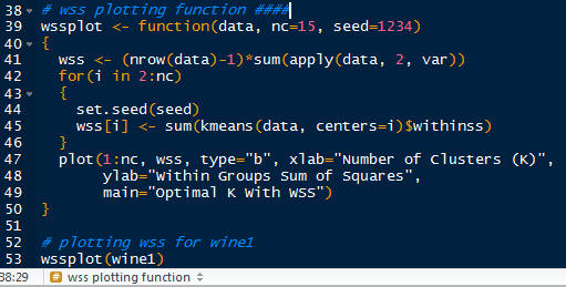
wssplot Code

This yields the within groups sum of squares plot for each k value:

Within Group Sum of Squares by Cluster Number

We see that the 'elbow' where the sum of squares stops decreasing drastically is around 3 clusters, then the decrease tapers off. This is our k value!

The NbClust is a package dedicated to finding the number of clusters by examining 30 various indices. We set the minimum number of clusters at 2 and the maximum at 15.

NbClust Code

The table will yield the clusters chosen by the criteria. Note not all of the criteria could be used. As we can see, 3 clusters had the overwhelming majority.

Clusters Chosen by Criteria

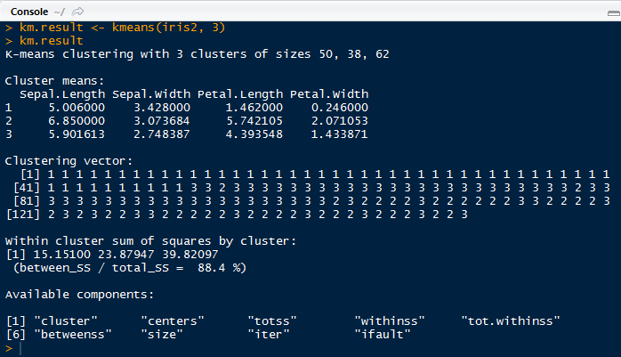
These are just some ways in which we can obtain the optimal k value before starting the kmeans clustering. The kmeans output is shown below in aggregate(), with k = 3.

Variable Averages in Each Cluster

We can check how well the kmeans clusters =3 clustered the data by using the flexclust package. See how well the clustering was for wine types 2 and 3? Not very well with a low index of 0.371.

Wine Table and Index

In following posts, we will cover hierarchical clustering. So stay tuned!



Thanks for reading,


Wayne
@beyondvalence
LinkedIn
(link)

Cluster Analysis: Using K-Means in R

Hello Readers,



Hope you guys are having a wonderful holiday! (I am.) Today in this post we will cover the k-means clustering technique in R.

We will use the familiar iris data set available in R.


Let us get started!

K-Means Clustering

Start by loading the cluster package by library(cluster) in R. The first and very important step in k-means clustering occurs when choosing the number of final clusters (k). 

Therefore the k-means clustering process begins with an educated 'guess' of the number of clusters. With the k number of clusters, R selects k observations in the data to serve as cluster centers. Then the Euclidean distance is calculated from observations to the cluster centers, and the observations are placed in the cluster to which they are closest.

Then the center of each cluster is recalculated and the Euclidean distance is taken for each observation and the new cluster center. R checks every observation to see if it is closer to another cluster center and reassigns it if it is closer to another cluster. The process of center cluster recalculation and observation distance checking is repeated until observations stay in the same cluster.

The kmeans() function requires the choosing k observations as the centers of the clusters.

Before clustering, remove the species column from the iris data set to retain the numerical values only.

Iris2 Data Set Without Species

Now use the kmeans() function on iris2 with 3 centers, or number of clusters, as shown below with the output.

K-Means Result

Note that the output includes the size of each cluster (50, 38, 62), the means of each variable in each cluster, the vector of the cluster number, the withinss for each cluster, and the components of the km.result object.

kmeans() seeks to minimize the withinss for each cluster, which is the sum of of squared error (SSE) or scatter. It is calculated by taking the sum of the squares of the distances between the observations and centroid of each cluster.

To see how well the k-means clustering performed, we can create a table with the actual species of iris and the cluster numbers:

Species and Cluster Comparison

As we can see, the clustering successfully clustered all the setosa species, but had difficulty with virginica (14 off) and versicolor (2 off). To quantify the agreement we can use the the library(flexclust) package, as shown below:

Adjusted Rank Index

An agreement of 0.73 is not too bad, as it ranges from -1 (no agreement) to 1 (perfect agreement). We have a 0.73 agreement between the iris species and cluster solution.

Plotting Clusters

Next we can visualize the clusters and their centers we constructed, with the code below:

Plotting Code

And that yields the visual below. Note that the three diamonds are the cluster centers in black, green and red.

Iris Clusters Plot

The model looks OK, except for a few red cluster points close to the green center, possibly miss classification of the virginica and versicolor species, because setosa was completely categorized properly. As we can see, the clustering is not perfect, hence an agreement score of 0.73.


In the next Cluster Analysis post I will discuss finding a suitable k to begin the k-means analysis. In this case, we knew we had 3 species to begin, so it was easy to plug in the k. However, we will look at the within sum of squares and sets of criteria to see what k we will use for a data set on wine. Stay tuned!


Thanks for reading,


Wayne
@beyondvalence