Sochi #Olympics and #Crimea Tweets in R (and Justin Bieber?!)

Hello Readers,


With the 2014 Olympics in Sochi over, we can reflect upon the social media coverage in the Olympic Games. What were Twitter users tweeting about that involved #Olympics during the games? And read on to see how Justin Bieber pops up (I was confused/surprised too).

In other news across the pond, if you have not been stuck in a cave recently, you might have heard about Russian forces 'occupying' the southern Ukrainian island of Crimea. And here is a series of informative satellite images of Crimea and military force disposition around Ukraine. We will see what Twitter users are talking about concerning #Crimea.

The twitteR package in R has many interesting features which we will use to query tweets from the newly modified Twitter API. So be sure to double check your unique consumer and secret keys, though they should not have changed. Also verify that the URLs used in the OAuth generation includes https://, and not just http://. 

Let us see what Twitter users have been tweeting about the Olympics and Crimea. Onward with text analysis!

Querying Tweets

In previous posts I covered retrieving tweets from the Twitter API, and transforming them into documents to be analyzed. So here I will simply show the R code,  beginning with establishing a handshake with the Twitter API (use https:// with recent changes). 

Setting Up OAuth

During some of the times I queried tweets I found that the number of tweets returned from the API varies from 25 to 199, even if n was set at 300. A way around was to query multiple times and join the resulting tweets together. I had no problem with the Olympics tweets however, but they were queried weeks ago during the games.

Give Me More Tweets!

For the Olympics tweets the code would simply be:

olympics <- searchTwitter("#Olympics", n=300)

Text Transformations

Next we would convert the lists to data.frames, and then to a text corpus. After they are in a text corpus, we can transform the text so we can query the words effectively. The crimea.c transformations similar to the olympics.c so they are omitted.

Raw Lists to Transformed Text Corpus

Now we are ready to normalize the text so that we can count their frequencies, and turn them into term document matrices.

Word Stemming and Term Doc Matrix

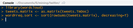
From the term document matrix, we can calculate the frequency of terms across all tweets. For example, from the crimea.tdm tweets, we can print the words occurring more than 20 times:

High Frequency Words in Crimea Tweets

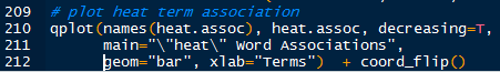
The next step would be to visualize these frequencies in a word cloud. #Olympics is up first.

#Olympics

In a previous post, we created a word cloud visualizing words from @nbastats. Here we shall do the same for the trend #Olympics.

Creating a Word Cloud

And here it is!

#Olympics Word Cloud

We see olympics, gold, sochi, and other strange terms such as jeremybieber (what!?). Who is Jeremy Bieber? An athlete? I had no idea, so I Google searched him, and he is definitely not an athlete. Apparently he is the father of 'notorious' pop star Justin Bieber. Some celebrity drama was unfolding during the Olympic Games and people flew to Twitter to comment. But it was weird (for me anyways) that music celebrities would be included in the same tweet tagged with #Olympics.

Upon more digging with Google, I found possible reasons: ice hockey and Canada. So the Beibers are originally from Canada and many Justin Bieber 'haters' want him to go back to Canada. With the American and Canadian hockey teams facing off at the Olympic semi-finals, this billboard popped up in Chicago:

Loser Keeps Bieber

So there was the cause for all the hullabaloo on Twitter. Unfortunately, so the 'haters', Justin stays because the USA men's hockey team lost to Canada's team 1-0 in the semi-finals. I could not make this up.

#Crimea

For Crimea (Bieber is not Ukrainian too, is he?), the word cloud code is the same, except change the *.tdm to crimea.tdm. And here is is:

#Crimea Word Cloud

We see many terms which associate with Crimea, such as ukraine, russia, putin, referendum, kiev, and etc., and also some Ukrainian terms as well- kyiv (Kiev, the Ukrainian capital). The majority of people in Crimea are Russian, while many in Western Ukraine are Ukrainian, wanting to join the EU. Crimea previously held a referendum for joining Russia in 2004 and would held another one today March 6th, 2014. The local lawmakers in Crimea voted unanimously in a referendum to join Russia, and would hold a regional vote in 10 days. For a video on the history of Crimea/Ukraine/Russia, click here.

I thought the terms in #Crimea were more logical and politically relevant than terms in #Olympics, although it was amusing to see Justin and his dad mentioned.

___________________________

Hopefully this post shows you how Twitter keywords or trends can be analyzed and visualized, especially when current events are concerned. It is near real-time text data of what people thinking about, and it is easy to analyze the tweets using R. Stay tuned for more R posts!



As always, thanks for reading,


Wayne
@beyondvalence

Text Mining: 4. Performing Term Associations and Creating Word Clouds in R

Hello Readers,




Welcome back to my blog. Today we will discuss analysis of a term document matrix that we created in the last post of the Text Mining Series. 

We will perform frequent term searches, and terms associations with visualizations. Then we finish the post by creating a visual word cloud (to the right) to 'display' the content of the terms in the tweets from @nbastats. Read Part 5 here.


Start R and let us begin programming!

Plotting Word Frequencies

Here we continue from where we left off last time. Begin by loading the twitteR, tm, and ggplot2 packages in R. Using the findFreqTerms() function in the tm library to find the most frequent terms. We can specify the lower and upper bounds of the frequency values using lowfreq and highfreq. Here we return terms with 20 or more occurrences.

High Frequency Terms

Next we take the 17 terms and create a bar graph of the frequencies using ggplot2. We can obtain the term counts by using rowSums() and we subset the sums to return values 20 or greater. Then we can plot the graph using qplot(), and the geom="bar" argument will create the bar graph, the coord_flip() flips the x and y axis.

Bar Graph Code

The neat result is shown below:

Term Frequencies

We can see that "games", "last", and "amp" are the top three terms by frequency.

Finding Word Associations

Using word associations, we can find the correlation between certain terms and how they appear in tweets (documents). We can perform word associations with the findAssocs() function. Let us find the word associations for "ppg" (points per game) and return the word terms with correlations higher than 0.25.

Associated Terms for "ppg"

We see that "ppg" has a high 0.65 correlation with "rpg", or rebounds per game. This makes sense as a tweet which contacts statistics about the points per game would also include other statistics like rebounds as well as "apg"- assists per game and "fg" field goals.

What about a team, say the Heat which has LeBron James? We can find the word associations for "heat":

Word Associations for "heat"

The top correlated terms are "adjusts", "fts" (free throws), "rockets", "thunder", and "value". Both the Houston Rockets and the Oklahoma City Thunder at top teams so it makes sense that there would be mentions of top teams in the same tweet, especially if they play against each other. LeBron is having a record year in player efficiency which might be why "trueshooting" is an associated term with 0.49 correlation for true shooting percentage.

We can plot the word associations for "heat". The code, similar to the previous plot, is shown below.

Plotting "heat" Word Associations

Which yields:

"heat" Word Associations

And there we have the word associations for the term "heat". I think that is a nice looking visual.

Creating a Word Cloud

We are going to continue the visual creation spree, and this time we will create a word cloud. Load the wordcloud package in R and convert the tweet term document into a regular matrix. 

wordcloud, Matrix Conversion, and Sorted Word Frequencies

After we created a word count of all the terms and sorted them in descending order, we can proceed to making the word cloud. We will set a set seed (at 1234) so that the work is reproducible. We need to create a gradient of colors (this time in gray) ranging from 0 to 1 for the cloud, based on the frequency of the word. More frequent terms will have darker font in the word cloud.

With the wordcloud() function, we can create the word cloud. We need to specify the words, their frequencies, a minimum frequency of a term for inclusion, and the color of the words in the cloud.

Word Cloud Plot Code

The word cloud is shown below!

Word Cloud for @nbastats

So in this post we have performed word associations for high frequency terms in our tweet term document matrix. We have also created a visualizations for the word associations and a word cloud to visualize the top occurring terms in the term document matrix for tweets from @nbastats.

Stay tuned for more analysis for hierarchical clustering of the terms!


Thanks for reading,

Wayne
@beyondvalence
LinkedIn