Up, Up, And Away: Amazon Stock Prices in R

Hello Readers,

Today we turn to the world of finance as we look into stock prices, specifically that of Amazon, Inc (AMZN). AMZN has been traded on the NASDAQ stock exchange since their IPO on May 15th, 1997  at 18.00 per share. Nowadays in 2014, AMZN trades around 369 dollars a share. Quite a long ways from a simple book selling company in Jeff Bezo's garage. I am sure Jeff Bezos is smiling. A lot.

Jeff Bezos, Founder and CEO/Chairman/President of Amazon

At the Yahoo Finance site, we can download AMZN stock price data, such as the opening price, the high and low of the day, closing price, and the volume (number of stocks bought and sold). Check the beginning date is March 3, 2008, the end date is March 12, 2014 (when I retrieved the data), and prices are set to monthly. Then at the bottom of the chart, there is a 'Download to Spreadsheet' CSV link (or just click the link).

Download AMZN Prices from Yahoo Finance

Now that we have the stock prices data, let us start number crunching to predict future Amazon stock prices in R.

AMZN in R

We need to import the CSV file into R. Locate the AMZN CSV file in your computer directory and write a read.csv() function pointing along the directory, making sure header=True. We will be using the closing prices.

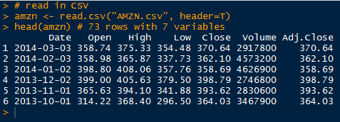
Reading in CSV and AMZN Data

We see from the first six rows in amzn, that the closing prices are in 5th column, and the prices are ordered from most recent to previous prices. When creating the time series, we need to reverse the 5th column, and specify the starting month and year with start=c(2008, 3). There are 12 monthly prices in a year so freq=12.

Creating AMZN Time Series and Data.frame

In addition to the single time series, we can manipulate the data by taking the log of the values and placing both into an accessible data.frame.

Next we plot the AMZN stock prices to get an idea of any trends in the prices over the 6 years.

Plotting Both AMZN and log AMZN Prices

Below we have the two plots, the AMZN stock price and the log of the AMZN stock price. We can see the obvious rise over the 6 years from 71.3 in March 2008 to 370.64 in March of 2014.

Observe the same upwards trend for the log of the stock prices. Note that fluctuations at lower values  (around 2009) tend to produce greater effect when log transformed, since the values are the exponents of base e.

Decomposition

There is a function, stl(), which decomposes the amazon time series into seasonal, trend, and remainder components. stl() finds the seasonal component through loess smoothing (or taking the mean if s.window="periodic"). The seasonal component is removed from the data and the remainder is smoothed to find the trend. The residual component is calculated from seasonal plus trend fit residuals. Use the stl() function to decompose the closing prices in amazon, and plot the result.

amazon Decomposition

See how variable the seasonal component is through the extreme values ranging from -5 to 10. There are also definitive peaks and valleys at specific times during the year. For example, in the 4th quarter (Q4- October, November, and December) this is a dramatic rise and fall in price by about 15 points.

Overall, the trend shown above depicts the expected upwards trend in stock price, besides the prices from 2008 into 2009, coinciding with the great financial collapse. Next we will use this output to forecast the price of AMZN stock in 2 years- March 2016.

Forecasting with stl()

Load the forecast package with the library() function. It enables us to forecast different time series models and linear models with the forecast() function. We specify our decomposed time series, amazon.stl, and determine our prediction method as "arima". Next we want to predict 24 periods into the future (or 24 months- 2 years), with a 95% confidence interval specified with level=95. Then we visualize our results by passing our forecast object through plot().

stl() ARIMA Forecasting AMZN

We see the resulting (wonderful) plot below. Observe the forecast prices modeled and determined by auto.arima as the blue line, shadowed by the 95% confidence interval in grey. (ARIMA was cover in this post.) The model forecasts a likely increase of the AMZN stock price over 400 through year 2016.

The forecast values for AMZN through 2016 are shown below. The forecast for AMZN in March 2016 is 470.42, with a 95% confidence interval of the actual value lying between 333.96 and 606.88.

Forecast AMZN Values

From that forecast, I would buy some AMZN stock! Especially after Amazon announced on March 14th that they would raise Amazon Prime membership by $20 to $99 a year for free two-day shipping, video streaming, and other features. Many analysts concluded this move would increase profits by millions and AMZN stock rose 1% (about 3.5 points). I am sure Jeff Bezos is smiling even more.

OK folks, hopefully now you have a better understanding of decomposition and forecasting time series! Check back for more analytic posts!


Thanks for reading,

Wayne
@beyondvalence

Time Series: 1. Decomposition into Components-Additive Model in R

Hello Readers,

Today we will discuss time series in this post. We will be using the AirPassengers data set available in R. It describes the monthly ridership of international airline passengers from 1949 to 1960. 

We will perform time series decomposition of the data to gain a better understanding of the airline passenger patterns (trend, seasonal, cyclical, long-term, residual, etc.) during that time. This is the first part of the 'Time Series' series (we will conduct series forecasting later).

Open R, and let us get started!

The Time Series Class

To begin, R has a class of objects especially for time series analysis. They are designated as ts (click me!), which are data sampled at equidistant points in time. Below is an example of a time series. It has values from 1 to 30, repeating 12 times indicating by month, starting from year 2011 in the third month, March. The attributes() tells us the properties of the time series and the class.

Sample Time Series

Call attributes() and str() on AirPassengers to see what we are working with. The attributes show the low and high time values (1949.000, 1960.917) followed by the interval between the data values (12.000). Usually an interval of 7 represents weeks, 12 means months, and 4 means yearly quarters, so here, the AirPassenger data is measured monthly.

Attributes and Structure of AirPassengers

Next, the structure informs us of the value numbers (1 to 144), the years (1949 to 1961), and then the actual passenger volumes, in thousands starting from 112, 118, 132, and so on. We can also visualize the data with a simple plot:

Basic AirPassengers Plot

Now that we have a good grasp of the ts() object and the data set we will analyze, it is time for the decomposition process.

Time Series Decomposition

Fantastic. But what is decomposition? Simply put, decomposition breaks down a time series into components- such as trend, seasonal, cyclical, and irregular (see Note at end). Trend refers to the long term trend, seasonal is seasonal variation- fall, winter, etc. Cyclical means repeated fluctuations, that are non-periodic, and the irregular component refers to abnormal fluctuations, also known as residuals.

• Time Series Data = Seasonal Effect + Trend + Cyclical + Residual

First, create another time series set with ts(), apts (short for AirPassengers Time Series) with a frequency of 12. This set will start at a default year 1 with the AirPassengers numbers. The decompose() function will yield a list containing the various components below. Take note of the class name.

apts Time Series Decomposition

The apts.de is a decomposed.ts class object, with various vector measurements of the components. For example, we can look at the estimated seasonal decomponent in apts.de$figure, and see that in the 11th month, November, there was a low seasonal factor of -53.59, and in July (7) there was a high seasonal factor of 63.83. It appears that airline ridership peaks in the summer and fall months and falls during the winter.

Plotting Seasonal Decomponent

Naturally, we can visualize the seasonal factors with the above code to yield a graphic. And yes, it looks as if the airlines are really popular in the summer- makes sense for vacation time (in North America)!  

Seasonal Factors

 We can also plot the all the components together with the observed time series in a single plot. Notice that the over all trend is increasing, the seasonal factor peaks during summers, and there is more fluctuation in the earlier and later years in the data than the middle. It is obtained after removing the long term trend, and seasonal factors from the data.

Decomponents Plot

Seasonal Factors Adjustment

Also, we can adjust the AirPassengers data now that we have some decomposition factors. Let us adjust for seasonality. Begin with the original AirPassengers data to have the years intact. Next, use the decompose() function to obtain the components. Next, subtract the seasonal factor from the original data into another data set and label it appropriately.

Seasonal Factors Adjustment Code and Plot

After plotting the adjusted data, we can observe how from the end of 1953 to middle of 1956 there is little fluctuation compared to the earlier and later years. Because we adjusted for seasonality, that means from '53 to '56 much of the fluctuation was due to differences in season, whereas the years prior to 1953 and after 1956, the fluctuations are not really influenced as much from season time. 

This is shown by how after the seasonal factors were removed from the time series, the ridership from 1953 to 1956 increased more stably. It appears that passengers were not influenced as much by the season in which to fly before 1953 and after 1956.

Note:

This decomposition assumes that the time series is calculated as an additive model as opposed to an multiplicative model, where the components are multiplied together. Multiplicative models are considered when the absolute differences are less important than the proportional differences in a time series. For example, if we had a time series of exponential growth of bacteria, or price inflation, the proportional change can be overlooked when the absolute values are smaller using an additive model. The decompose() function can be modified with a type="multiplicative" argument for a multiplicative model. The multiplicative model is shown below. We can just take the logarithms of each side and then the components act as an additive model.

• Time Series Data = Seasonal Effect * Trend * Cyclical * Residual
• Into:
• log( Data) = log(Seasonal Effect) + log(Trend) + log(Cyclical) + log(Residual)

And there we have it! This concludes time series decomposition for now. There are more advanced functions for time series, such as stl() which we will cover in later posts. But for now, the next post in the series will move on to time series forecasting.


Thanks for reading,


Wayne
@beyondvalence