#PublicHealth on Twitter in R

Hello Readers,

In this post we examine at a specific hashtag on Twitter: #PublicHealth. When I am not spending time studying analytics, I concentrate on the biostatistics and public health, which introduced me to data science.

Analytics plays an important role in public health, as evidence based decisions rely on proper data gathering and analysis for their scientific rigor. Data and information is the power to understand, especially in our times of technology and communication. For example, Google tapped into their search results related to flu symptoms, and managed to model and predict flu trends, which I covered in these two posts. So using Twitter, we can see snippets of public health mentions in what people are tweeting.

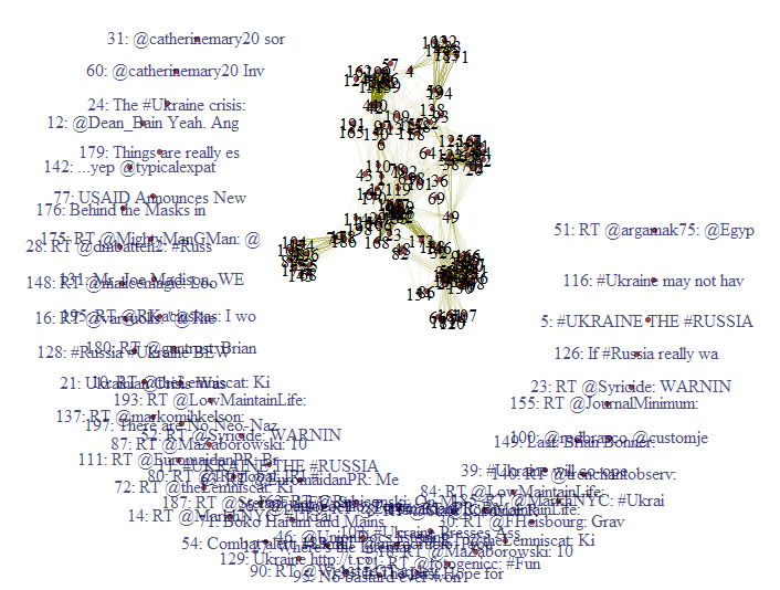
Because Twitter is a real-time micro-blogging site, we can take a snapshot of tweets for a specific user, topic, or time-frame. So here I chose to exhibit the topic #PublicHealth, in light of the ebola epidemic spreading in Western Africa. This particular outbreak is one of worst in history, occurring in Sierra Leone, Guinea, and Liberia with 982 cases and 613 deaths (as of July 17) since March of 2014. The Centers for Disease Control and Prevention (CDC) has sent specialists to track, contain, and inform the locals about the Ebola outbreak.

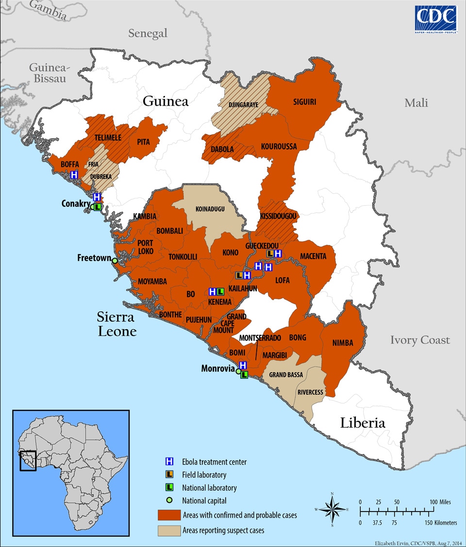
Ebola Map, by CDC

Returning back to Twitter and #PublicHealth, from the 300 tweets I queried in R, by using text transformation in R, I created a word cloud of the words in the tweets:

#Public Health

The querying from Twitter, text transformation, and word cloud creation code can be found in the Appendix, below. As we investigate the word cloud, aside from "publichealth", we see some terms, such as: 

• "croakeyblog", a blog about health,
• "profkevinfenton", Dr. Kevin Fenton, director of health and wellbeing at Public Health England,
• "data",
• "human",
• "ecigarettes",
• "healthcare",
• and "ebola" on the top left.

#PublicHealth covers a wide range of subtopics, and also links to many others as well. With increased globalization, and aging populations, both communicable and non-communicable diseases are rising across the world. Here is the World Health Organization (WHO) on immunizations, and reducing preventable deaths.

For those interested in studying or learning more about public health, consider the Johns Hopkins Bloomberg School of Public Health, and the Johns Hopkins Public Health Studies
undergraduate program. 


Thanks for reading,

Wayne
@beyondvalence
LinkedIn

Code Appendix:

Text Transformation Code:

1 2 3 4 5 6 7 8 9 10 11 12 13 14 15 16 17 18 19 20 21 22 23 24 25 26 27 28 29 30 31 32 33 34 35 36 37 38 39 40 41 42 43 44 45 46 47 48 49 50 51 52 53 54 55 56 57 58 59 60 61

> # load library > library(tm) > # > # transforming function (by Wayne) > # where x is text and w.stop is stopword vector, > # w.keep are words to remove from stopwords > # Term-Doc default, if false, then Doc-Term > transform.text <- function(x, w.keep=c(""), w.stop=c(""), TD=TRUE) { + + cat("Data has ", length(x), " documents.\n") + + cat("Beginning text transformation: \n\n") + + cat("Transforming to Corpus... (1/6)\n") + text <- x + text.corpus <- Corpus(VectorSource(text)) + + cat("Formatting Corpus... (2/6)\n") + # lower case + text.corpus <- tm_map(text.corpus, tolower) + # remove punctuation + text.corpus <- tm_map(text.corpus, removePunctuation) + # remove numbers + text.corpus <- tm_map(text.corpus, removeNumbers) + # remove URLs + removeURLs <- function(x) gsub("http[[:alnum:]]*", "", x) + text.corpus <- tm_map(text.corpus, removeURLs) + # add stopwords w + myStopWords <- c(stopwords('english'), w.stop) + # remove vector w from stopwords + myStopWords <- setdiff(myStopWords, w.keep) + # remove stopwords from corpus + text.corpus <- tm_map(text.corpus, removeWords, myStopWords) + + cat("Stemming Words... (3/6)\n") + # keep corpus copy for use as dictionary + text.corpus.copy <- text.corpus + # stem words #### + text.corpus <- tm_map(text.corpus, stemDocument) + + cat("Completing Stems... (4/6)\n") + # stem completion #### + text.corpus <- tm_map(text.corpus, stemCompletion, + dictionary=text.corpus.copy) + + if(TD==TRUE) { + cat("Creating T-D Matrix... (5/6)\n") + text.TDM <- TermDocumentMatrix(text.corpus, + control=list(wordLengths=c(1,Inf))) + cat("Text Transformed! (6/6)\n\n") + return(text.TDM) + } else { + cat("Creating D-T Matrix... (5/6)\n") + # create Doc-Term #### + text.DTM <- DocumentTermMatrix(text.corpus, + control=list(wordLengths=c(1, Inf))) + cat("Text Transformed! (6/6)\n\n") + return(text.DTM) + } + + }

Retrieving #PublicHealth Tweets Code:

1 2 3 4 5 6 7 8 9 10 11 12 13 14 15 16 17 18 19 20 21 22 23 24 25 26 27 28 29 30 31 32 33 34 35 36 37 38 39 40 41 42

> library(twitteR) > library(tm) > > # load twitter cred #### > load("cred.Rdata") > registerTwitterOAuth(cred) [1] TRUE > > # configure RCurl options > RCurlOptions <- list(capath=system.file("CurlSSL", "cacert.pem", package = "RCurl"), + ssl.verifypeer = FALSE) > options(RCurlOptions = RCurlOptions) > > # query twitter for #PublicHealth in tweets, n=300 #### > pH <- searchTwitter("#PublicHealth", n=300, lang="en", + cainfo=system.file("cacert.pem")) > save(pH, file="publicHealth.rdata") > > # to data.frame #### > pH.df <- do.call("rbind", lapply(pH, as.data.frame)) > # use textTransformation function #### > pH.tdm <- transform.text(pH.df$text, w.stop = c("amp", "rt") ,TD = TRUE) Data has 300 documents. Beginning text transformation: Transforming to Corpus... (1/6) Formatting Corpus... (2/6) Stemming Words... (3/6) Completing Stems... (4/6) Creating T-D Matrix... (5/6) Text Transformed! (6/6) > # find terms with n > 20 [1] "advice" "blogs" "can" "climate" [5] "cost" "croakeyblog" "data" "day" [9] "elderly" "eye" "falls" "health" [13] "heat" "heatwave" "helping" "herts" [17] "india" "issue" "jimmcmanusph" "keep" [21] "major" "need" "neighbours" "pheuk" [25] "please" "prevent" "profkevinfenton" "publichealth" [29] "stories" "support" "today" "vulnerable" >

Creating the Word Cloud Code:

1 2 3 4 5 6 7 8 9 10 11 12 13

> # generate word cloud #### > library(wordcloud) Loading required package: Rcpp Loading required package: RColorBrewer > pH.matrix <- as.matrix(pH.tdm) > wordFreq.sort <- sort(rowSums(pH.matrix), decreasing=T) > # wcloud > set.seed(1234) > grayLevels <- gray( (wordFreq.sort + 10) / (max(wordFreq.sort) + 10)) > wordcloud(words=names(wordFreq.sort), freq=wordFreq.sort, + min.freq=3, random.order=F, colors=grayLevels) >

Text Mining: 8. #Ukraine Tweet Network Analysis in R

Hello Readers,

Today we turn to tweet analysis in our Text Mining Series, as the last text mining post discussed term analysis. Instead of looking at how each individual word, or terms in each tweet relate to each other, we will visualize tweets as a whole and how they relate to each other based on their term similarity.

We will continue to use the #Ukraine tweets queried in the K-Medoids clustering post. You can following along with whatever trending twitteR query you prefer. Here we will go from a term-document matrix to a network object. Start R and let us get started.

#Ukraine Tweets as a Network

There were certain key terms in the tweets that connected the #Ukraine tweets together. Removing them would improve our ability to see underlying connections (besides the obvious), and simplify the network graph. So here I chose to remove "ukraine", "prorussian", and "russia".

You might remember last time to create an adjacency matrix for the terms, we multiplied the term-document matrix and its transpose together. Here we will perform the same matrix multiplication but in a different order, to create an adjacency matrix for the tweets (documents). This time we require the transpose of the tweet matrix multiplied by the tweet matrix, so that the tweets (docs) are multiplied together.

Tweet Adjacency Matrix Code:

# Tweet Network Analysis ####
load("ukraine.tdm.RData")

# remove common terms to simplify graph and find
# relationships between tweets beyond keywords
ukraine.m <- as.matrix(ukraine.tdm)
idx <- which(dimnames(ukraine.m)$Terms %in% c("ukraine", "prorussian", "russia"))
ukraine.tweetm <- ukraine.m[-idx,]

# build tweet-tweet adjacency matrix
ukraine.tweetm <- t(ukraine.tweetm) %*% ukraine.tweetm
ukraine.tweetm[5:10,5:10]

    Docs
Docs 5 6 7 8 9 10
  5  0 0 0 0 0  0
  6  0 2 0 0 1  0
  7  0 0 1 0 0  0
  8  0 0 0 0 0  0
  9  0 1 0 0 4  0
  10 0 0 0 0 0  0

We see from the tweet adjacency matrix, the terms two documents have in common. For example, tweet 9 has 1 term in common with tweet 6. The number will be the same whether you start at tweet 9 or tweet 6, and compare the other.

Now we are ready for plotting the network graphic.

Visualizing the Network

Again we will use the igraph library in R, and use the graph.adjacency() function to create the network graph object. Recall that V( ) allows us to manipulate the vertices and E() allows us to format the edges. Below we change and set the labels, color, and size for the vertices.

Tweet Network Setup Code:

# configure plot
library(igraph)
ukraine.g <- graph.adjacency(ukraine.tweetm, weighted=TRUE, mode="undirected")
V(ukraine.g)$degree <- degree(ukraine.g)
ukraine.g <- simplify(ukraine.g)

# set labels of vertices to tweet IDs
V(ukraine.g)$label <- V(ukraine.g)$name
V(ukraine.g)$label.cex <- 1
V(ukraine.g)$color <- rgb(.4, 0, 0, .7)
V(ukraine.g)$size <- 2
V(ukraine.g)$frame.color <- NA

# barplot of connections
barplot(table(V(ukraine.g)$degree), main="Number of Adjacent Edges")

Barplot of Number of Connections

From the barplot, we see that there are over 60 tweets which do not share any edges with other tweets. For the most connections, there is 1 tweet with 59 connections. The median connection number is 16.

Next we modify the the graph object even more by accenting the vertices with zero degrees selected by index in the idx variable.. In order to understand the content of those isolated tweets, we pull the first 20 characters of tweet text from the raw tweet data (you can specify how many you want).

Then we change the color and width of the edges to reflect a scale of the minimum and maximum weights (width/strength of the connections). This way we can discern the size of the weight relative to the maximum weight. Then we plot the tweet network graphic.

Plotting Code:

# set vertex colors based on degree
idx <- V(ukraine.g)$degree == 0
V(ukraine.g)$label.color[idx] <- rgb(0,0,.3,.7)
# load raw twitter text
library(twitteR)
load("ukraine.raw.RData")
# convert tweets to data.frame
ukraine.df <- do.call("rbind", lapply(ukraine, as.data.frame))
# set labels to the IDs and the first 20 characters of tweets
V(ukraine.g)$label[idx] <- paste(V(ukraine.g)$name[idx], 
                                 substr(ukraine.df$text[idx], 1, 20),
                                 sep=": ")
egam <- (log(E(ukraine.g)$weight)+.2) / max(log(E(ukraine.g)$weight)+.2)
E(ukraine.g)$color <- rgb(.5, .5, 0, egam)
E(ukraine.g)$width <- egam
layout2 <- layout.fruchterman.reingold(ukraine.g)
plot(ukraine.g, layout2)

Initial Tweet Network Graphic

The first 20 characters of tweets with no degrees in blue surround the network of interconnected tweets. Looking at this cumbersome graphic, I would like to eliminate the zero degree tweets so we can look at the connected tweets.

Revised Plotting Code:

# delete vertices in crescent with no degrees
# remove from graph using delete.vertices()
ukraine.g2 <- delete.vertices(ukraine.g, 
                              V(ukraine.g)[degree(ukraine.g)==0])
plot(ukraine.g2, layout=layout.fruchterman.reingold)

Tweet Network Graphic- Removed Unconnected Vertices

Now with the degree-less tweets removed, we can get a better view of the tweet network. Additionally, we can delete the edges with low weights to accentuate the connections with heavier weights.

Revised Again Plotting Code:

# remove edges with low degrees
ukraine.g3 <- delete.edges(ukraine.g, 
                           E(ukraine.g)[E(ukraine.g)$weights <= 1])
ukraine.g3 <- delete.vertices(ukraine.g3, 
                              V(ukraine.g3)[degree(ukraine.g3)==0])
plot(ukraine.g3, layout=layout.fruchterman.reingold)

Tweet Network Graphic- Removed Low Degree Tweets

The new tweet network graphic is much more manageable than the first two graphics, which included the zero degree tweets, and edges with low weight. We can observe a few close tweet clusters- at least six.

Tweet Clusters

Since we now have our visual of tweets, and see how they cluster together with various weights, we would like to read the tweets. For example, let us explore the cluster in the very top right of the graphic, consisting of text numbers 105, 177, 145, 152, 68, 89, 88, 55, 104, 174, and 196.

Code:

# check tweet cluster texts
ukraine.df$text[c(105,177,145,152,68,89,88,55,104,174,196)]

 [1] "@ericmargolis Is Russia or the US respecting the sovereignty and territorial integrity of #Ukraine as per the 1994 Budapest Memorandum????"      
 [2] "Troops on the Ground: U.S. and NATO Plan PSYOPS Teams in #Ukraine - http://t.co/pXP3TR0uwi #LNYHBT #TEAPARTY #WAAR #REDNATION #CCOT #TCOT"       
 [3] "US condemns ‘unacceptable’ Ukraine violence http://t.co/OcAClP01sF #Ukraine #Russia #USA #USAOutOfUkraine #MaidanDictatorship #Terrorism"    
 [4] ".@Rubiconski  Apparently there's a treaty w US that if #Ukraine got rid of nukes, US would protect them."                                        
 [5] "Unsurprisingly no one has made a comparison to #stalin about #dissidents losing native status in #ukraine. http://t.co/OylSNE6vAi #OSCE #US"     
 [6] "RT @Yes2Pot: .@Rubiconski  Apparently there's a treaty w US that if #Ukraine got rid of nukes, US would protect them."                           
 [7] "Ukraine violence reaches deadliest point as Russia calls on U.S. for help #Ukraine. http://t.co/CqvVmkiltR http://t.co/OMQ8Cx6tOO"               
 [8] "RT @cachu: Ukrainian passports to Polish #mercenaries to fight against UKRAINIANS   - http://t.co/Z1IoX051Jo… #Poland #Ukraine #Russia #US …"
 [9] "More U.S. #Sanctions Pledged Should #Ukraine Crisis Persist: The U.S. may impose… http://t.co/pF77x4GzLh"                                      
 [10] "RT @MDFoundation: LNG exports from the U.S. can make Ukraine and even Europe more independent http://t.co/hQmNB5V93R #LNG #Ukraine #Russia …"  
 [11] "#Ukraine to Dominate Merkel's U.S. Visit - The Ukraine crisis—and the role of further potential... http://t.co/rwnHqoduFR\n #EuropeanUnion"

What a wall of text! So these 11 tweets have many terms in common with each other with the common terms removed. Although they all have to do with #Ukraine, the topics vary from Merkel's visit in tweet 11, to the 1994 Budapest Memorandum in tweet 1, and NATO in tweet 2. You can go ahead and check the other clusters in your tweet network for text content.

So there we go, we have our tweet network visualization (as opposed to term network), and we can view specific tweets that we located through the visualization. Stay tuned for more R posts!


Thanks for reading,

Wayne
@beyondvalence
LinkedIn

Text Mining: 7. Term Network Analysis Using #Ukraine Tweets in R

Hello Readers,

Today we move to the next phase of text mining: network analysis of terms, or keywords from Twitter. This post will continue to use the #Ukraine tweet data from Twitter from the Text Mining 6: K-Medoids Clustering in the Text Mining Series.

So far we have covered hierarchical clustering, and k-medoids clustering, to group and partition the frequent words in tweets. With network analysis, not only can we determine which terms appear together frequently, we can visualize how keywords and tweets are connected as a network of terms. This way, we can resolve the number of connections keywords have with one another, and how many connections a specific keyword has with other keywords. 

Resulting Network of Terms

Using network terminology, our keywords are the 'nodes' in a network, which are called vertices. Connections are named edges. For an example using car makers, let us say the keyword "generalmotors" has a connection to both "ford" and "toyota". The vertex (singular of vertices) is "generalmotors", which has 2 edges linking it with "ford" and "toyota". Both "ford" and "toyota" are vertices as well, and could have other edges with other keywords connected or not connected to "generalmotors", such as "fiat" or "bmw".

Go ahead and load the igraph package in R, and let us begin.

#Ukraine Tweet Terms as a Network

Since we are using the tweet term data from the previous text mining post, we need to take the term document matrix and transform it into a matrix. Next we need to transform it into a Boolean matrix such that it indicates 0 or 1 for existing values other than zero. Therefore, we are just modifying the matrix to indicate yes or no for the term existing in a document.

Code:

# Network analysis

# load ukraine tdm data
load("ukraine.tdm.RData")

# create matrix
ukraine.m <- as.matrix(ukraine.tdm)

# to boolean matrix
ukraine.m[ukraine.m>=1] <- 1

# to term adjacency matrix
# %*% is product of 2 matrices
ukraine.m2 <- ukraine.m %*% t(ukraine.m)

The second matrix we create will show how many 'connections' each term has in a adjacency matrix. This will require the product of two matrices, using the '%*%' matrix operator. Through the inner product of the terms, we will arrive at the number of times each term appears together in a document.

Adjacency Matrix

Now that we have your adjacency matrix, we can go ahead and plot a network graph using the igraph package, after simplifying the graphic, and setting the labels and degrees of the vertices- the terms.

Plot Code:

# build graph with igraph ####
library(igraph)
# build adjacency graph
ukraine.g <- graph.adjacency(ukraine.m2, weighted=TRUE, mode="undirected")
# remove loops
ukraine.g <- simplify(ukraine.g)
# set labels and degrees of vertices
V(ukraine.g)$label <- V(ukraine.g)$name
V(ukraine.g)$degree <- degree(ukraine.g)

# plot layout fruchterman.reingold
layout1 <- layout.fruchterman.reingold(ukraine.g)
plot(ukraine.g, layout=layout1, vertex.size=20, 
     vertex.label.color="darkred")

Remember, the labels are the names of the vertices, and the degrees are the number of connections to other terms. We create a layout using the layout.fruchterman.reingold() function. In the plot() options, I specified a larger vertex size (vertex.size=20), and a darker label color (vertex.label.color="darkred") so we can see the terms better:

Ukraine Terms Network Graphic

We can observe "ukraine" being the central term holding the network together (being the term we used to query the tweets). Looking closer at the connections, we see other terms with many connections such as "southeastern", "prorussian", "odessa", and "observes". With the unrest occurring in the southeast by pro-Russian forces, among them in major city of Odessa, people are observing "dozens" "dead", and are in "mourning".

Luckily, there is a way of modifying the igraph object using the label size, label color, vertex border, and connection line size to make it easier to view the terms and connections. Note that for the label size ($label.cex), color ($color), and connection width ($width) are all determined by a percentage of the maximum vertex connections ($degree and E(ukraine.g)).

Improved Plot Code:

# change label size of vertices (nodes) V()
# change the edge color (connections) E()
V(ukraine.g)$label.cex <- 2.2 * V(ukraine.g)$degree / max(V(ukraine.g)$degree) + .2
V(ukraine.g)$label.color <- rgb(0, 0, 0.2, 0.8)
V(ukraine.g)$frame.color <- NA
egam <- (log(E(ukraine.g)$weight) + .4) / max(log(E(ukraine.g)$weight) + .4)
E(ukraine.g)$color <- rgb(.5, .5, 0, egam)
E(ukraine.g)$width <- egam
# improved plot
plot(ukraine.g, layout1)

We now can see the the terms more clearly:

Improved Term Network Graphic

With our new term colors and connections colors, they reflect the number of connections (degrees) each term has with other terms. Thus, we see definite terms that occur together (more connections-degrees) in tweets with larger labels and darker edges (lines). We see popular vertices (other than "ukraine")  in "observes", "east", and "prorussian". 

In the terms on the lower right,  "observes", "dead", "southeastern", "rtcom", "mourning", "days", "dozens", and "crimea", are highly interconnected, indicating that these terms tend to occur together in the same tweet.

There are more inferences you can draw from the #Ukraine term network visual, such as connections of terms to "prorussian". We see that it is heavily connected to "russia", "east", "forces", "foxnews", and "offensive".

On the right hand side, we see the city of "odessa". There have been heavy military activity and rioting, with pro-Russian activists being targeted in the chaos. Russia has equated the attacks with Russian ethnic genocide, which is why "nazis" appeared in the terms connected to "odessa".

Next we will move to network analysis on complete tweets, not just terms in tweets. So stay tuned more more #rstats!


Thanks for reading,

Wayne
@beyondvalence
LinkedIn

Text Mining: 6. K-Medoids Clustering of #Ukraine Tweets in R

Hello Readers,

Today we will continue the text mining series with a post on k-medoids clustering in R. For this analysis I queried 200 recent tweets (May 3rd) using the hashtag #Ukraine, considering the recent escalation of Ukrainian and pro-Russian forces in eastern Ukrainian cities.

You can catch up on the recent Ukraine Crisis in my previous post illustrating events and palladium prices. While we see that international economic sanctions threatening the supply of the rare metal from Russia reflected in the price, what has been the online Twitter reaction to the increasing conflict in the region? To assess online sentiment, we can look to tweets containing the #Ukraine hashtag.

Tweet Retrieval

For those of you who have difficulty in using the twitteR package in R, remember to change the URLs to https:// from http://. I had saved my handshake completed OAuth object from earlier posts, so I simply registered the credential object again.

Because this post will focus on k-means clustering, I will only post the R code, as my other text mining posts explain the tweet/timeline retrieval process.

Code:

require(twitteR)
require(OAuth)

# load twitter cred
load("cred.Rdata")
registerTwitterOAuth(cred)

# search twitter for ukraine tweets
ukraine <- searchTwitter("#Ukraine", n=200, lang="en", cainfo="cacert.pem")

# tm ukraine data ####
library(tm)
# to data.frame
ukraine.df <- do.call("rbind", lapply(ukraine, as.data.frame))
# to corpus
ukraine.corpus <- Corpus(VectorSource(ukraine.df$text))
# begin transformations
ukraine.corpus <- tm_map(ukraine.corpus, tolower)
ukraine.corpus <- tm_map(ukraine.corpus, removePunctuation)
ukraine.corpus <- tm_map(ukraine.corpus, removeNumbers)
removeURLs <- function(x) gsub("http[[:alnum:]]*", "", x)
ukraine.corpus <- tm_map(ukraine.corpus, removeURLs)
myStopWords <- c(stopwords('english'), "via", "rt")
ukraine.corpus <- tm_map(ukraine.corpus, removeWords, myStopWords)
# stem and replacement
ukraine.corpus.c <- ukraine.corpus
ukraine.corpus <- tm_map(ukraine.corpus, stemDocument)
ukraine.corpus <- tm_map(ukraine.corpus, stemCompletion,
                         dictionary=ukraine.corpus.c)
# to tdm
ukraine.tdm <- TermDocumentMatrix(ukraine.corpus, 
                                  control=list(wordLengths=c(1, Inf)))
# remove sparse terms
ukraine.tdm <- removeSparseTerms(ukraine.tdm, sparse=0.95)

The remaining terms, not removed by their sparsity, have more than 5% existing in documents:

Terms

Very quickly we can create a word cloud from the terms using the wordcloud package:

Code:

# wordcloud
library(wordcloud)
ukraine.m <- as.matrix(ukraine.tdm)
wordFreqSort <- sort(rowSums(ukraine.m), decreasing=TRUE)
grayLevels <- gray( (wordFreqSort + 10) / (max(wordFreqSort) + 10))
word.cloud <- wordcloud(words=names(wordFreqSort), freq=wordFreqSort, 
                        min.freq=3, random.order=F, colors=grayLevels,
                        scale=c(4.5,.9), rot.per=.1)

#Ukraine Word Cloud

We can see major terms in the word cloud in larger font aside from "ukraine", such as "russia", "odessa", "prorussian", "crimea", and others.

K-Medoids Clustering

Now that we have an idea of the terms from the #Ukraine tweets, and visually from the word cloud, we would like to determine how terms are associated with each other using k-medoids clustering. Which terms are closest to each other, such that they can be partitioned as clusters of terms?

To do so, we use the pamk() function from the fpc package, which will give the optimal cluster number via the average silhouette width (higher = better). pamk() is a wrapper function for the (more robust than k-means clustering) pam() function. PAM stands for "Partitioning Around Medoids". K-medoids uses data points as centers of clusters. It is more robust because it uses pairwise dissimilarities rather than the sum of squared Euclidean distances (vulnerable to outliers).

library(fpc)

# create a transposed matrix from tdm
ukraine.m <- as.matrix(ukraine.tdm)
ukraine.m2 <- t(ukraine.m)

# pamk clustering
ukraine.pam <- pamk(ukraine.m2, metric="manhattan")
# optimal cluster number
ukraine.pam$nc
[1] 2
# isolate cluster object
ukraine.obj <- ukraine.pam$pamobject
# print out terms in each cluster
for(i in 1:ukraine.pam$nc) {
+ cat(paste("cluster ", i, ": ", sep=""))
+ cat(colnames(ukraine.obj$medoids)[which(ukraine.obj$medoids[i,]==1)], "\n")
+ }
cluster 1: ukraine 
cluster 2: crimea days dead dozens mourning observes rtcom southeastern ukraine 

# plot clusters and silhouette
plot(ukraine.obj)

We see from the average silhouette width, the optimal cluster number is 2. Keeping that in mind, we want to observe which terms are in the two clusters. A for loop will accomplish what we would like to see: cluster 1 contains "ukraine", and cluster 2 contains the other terms, "crimea", "days", "dead", "dozens", "mourning", and etc.

Cluster Plot:
Our results are not fantastic coming from 199 tweets, but the two components explain ~37.57% of the variability. You can observe the clusters below- only 1 is distinct.

Silhouette Plot:
A silhouette width close to 1 indicates a good fit in the cluster (close together), whereas a lower value close to zero means the point is bordering 2 clusters, and a negative value indicates the point most likely is misclassified. The first cluster we have a decent average width of 0.65 for "ukraine", but for cluster two, we see a very high average width of 0.98 for the 9 terms.

What do these results mean? Well, it seems from the terms in the clusters, "ukraine" was used in tweets by itself most of the time. However, some of those tweets included more detail about the region of "prorussian" forces invading "crimea" or "southeastern" "ukraine". Those tweets tended to be similar to each other. So from the clusters, we determine that tweets with #Ukraine, are similar that they include only "ukraine" or "ukraine" and other comparable terms describing the crisis.

Stay tuned for more text analysis!


Thanks for reading,

Wayne
@beyondvalence
LinkedIn