Text Mining: 2. Converting Tweet Text List into a Document Corpus with Transformations Using R

Welcome Back Readers,



Last time in the Text Mining Series we discussed how to retrieve tweets from the Twitter API with the twitteR package in R. Now that we have the text data to work with, we can now transform the text from their raw format into a corpus, which is a collection of text documents.

This post continues from where we left off in Text Mining 1. Read Text Mining 3 here. We require the packages: tm for text mining and SnowballC for word stemming to collapse words.

Now is a good time to download and load them in R- so let us get started! 

Data.Frame to Corpus

As we saw from last time, the raw text in the tweet list object was far from polished and would take some formatting to clean. We start with converting the tweet list object into a data.frame after we load the packages and set the working directory:

Tweet List Object into Data.Frame Object

As we can see, the dimensions of the tweets data.frame has 186 rows and 16 columns. The descriptions for each column are shown below:

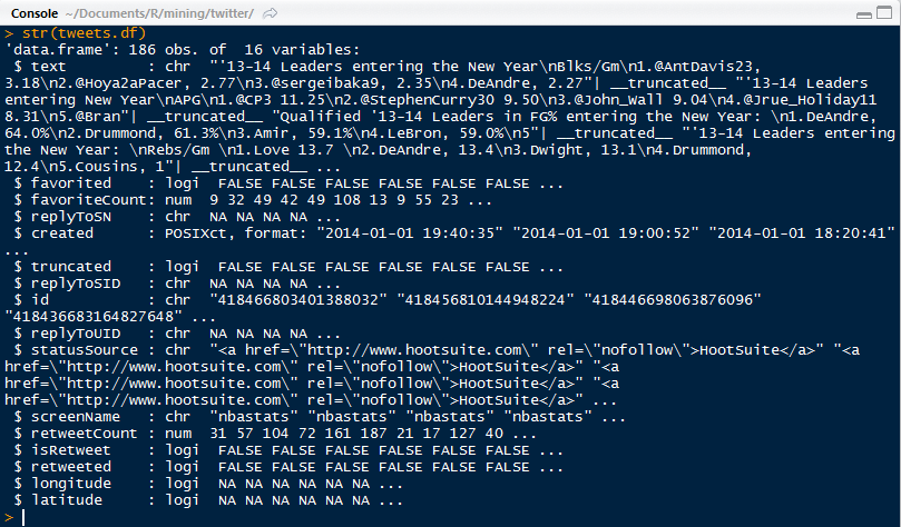
Tweet Data.Frame Column Structure

We have columns for the tweet text, whether the tweet is favorited by the user (my account since my app accessed it), how many favorites if any, tweet ID, and so on. Note at the bottom, there are yes/no for longitude and latitude coordinates- so we can track the location where the tweet was sent.

Now that the data exists as a data.frame, we can convert it into a corpus using the Corpus() function from the tm package (the link opens to a pdf of the tm package).

Tweets into Corpus

Observe that the corpus list has 186 text documents, which means that the conversion process converted each tweet into a text document. 

Next, we will transform the tweet corpus and the getTransformations() function displays the text transformations available for the tm_map() function in the text mining package. We have various transformations at our disposal, such as removing punctuation and removing numbers, words, and white space.

Transforming Text

First we will perform the following modifications using the tm_map() function: lowering character case, removing punctuation, removing numbers, and removing URLs. These are completed using the respective commands: tolower, removePunctuation, removeNumbers, and a regular expression substitution using gsub().

Removing Case, Punctuation, Numbers and URLs

The gsub() function allows us to replace the regular expression for an URL link, "http[[:alum:]]*" with "", a non-space for removal. Then we pass that function to the tm_map().

Adding and Removing Stopwords

Next we add stopwords. They are words that are ignored from searches with specific relevant topics and keyword combinations, increase the 'content' of the the tweet, and efficiency of analysis. They include, a, the, for, from, who, about, what, when, where, and more, depending on the analysis. Common stopwords, some even from Google Search filters out can be found here.

We can observe the changes of the text transformation, when we look at a random tweet. Say tweet #4 below. Note how all the punctuation was removed, as with the numbers, and newline escapes "\n", and that all characters are lowercase.

Tweet 4 Before and After

Next time around we shall discuss stemming the documents in the corpus we created and transformed in this post. Stemming involves cutting words shorter to retrieve their radicals. That way we can count their frequency despite the word being spelled differently or being used in a different tense. For example- updated, updating, update are 'stemmed' to updat.

And that is for next time! So stay tuned!


Thanks for reading,


Wayne
@beyondvalence
LinkedIn

R: Regex Telephone Number Matching

Hello Readers,


Firstly, here is an encouraging message from President Obama, calling for more students to learn code! Hooray, SCIENCE!


Now back to the post. Here we shall discuss using regular expressions to match North American telephone numbers in RegExr. For matching text from HTML5, check out this post.

Usual telephone numbers include a three digit area code followed by a seven digit number sequence, which can be separated by hyphen, period or even spaces. Sometimes the area code can be enclosed in parenthesis as well. So how do we match and extract the numbers that we require? So we turn to the flexibility of Regular Expressions to describe the target string we want to match. We will be using RegExr program, found here. Let us get started.

RegExr

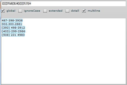
The picture of the RegExr window, above, shows a variety of telephone numbers, some separated with hyphens, some with periods, and others just with spaces. So how can we match the digits in the phone numbers? To demonstrate, we can first use:

1. Literal Strings

  By using the actual numbers, we can manually match the telephone numbers. For example, if we type 498, then RegExpr matches the sequence of digits 498 twice, as shown below.

RegExpr Matching 498

2. Shorthand

  By using the power of regular expressions, we can incorporate shorthand, which is a special type of character. A backlash lowercase d denotes any digit. The opposite is true when the d is capitalized to D, as any character that is not a digit is matched, such as hyphens, periods, parenthesis, etc. Both are shown below.

Matches Any Digit- Shorthand

And the reverse (conveniently the capitalized letter D):

Matches Any Non-Digit- Shorthand

3. Quantifiers

Since telephone numbers follow a pattern of 3 digits, 3 digits, and 4 digits, we can tell the match to loop for a certain amount of times by using a quantifier. For example, using curly brackets {n} to surround a number after a regular expression will instruct RegExr to match that expression n times. This is shown below, as \d (any number) is matched exactly three times. Note how in the last set of 4 digits, only the first 3 are matched.

Shorthand Matching with a Quantifier

To match the set of 4 numbers as well, we can use {n1, n2} as a quantifier where RegExr will match expression from the range n1 to n2. Additionally, the quantifier ? matches 0 or 1 of the preceding token, whereas the + will match 1 or more. The asterisk * will match 0 or more times.

More Quantifiers- It Works!

The ? after both parenthesis allow them to match when they are and are not there, so it will match the area code as well as the other digits in the phone number. The digit sets are set to match {3, 4} three to four times, and the optional period will match any character, whether it be a hyphen, period, or white space. Then the whole expression has to match at least once or more with the + sign.

4. Putting It Together


However, there are many different ways to match a specific string. Below is another method which uses anchors.

Simply put, anchors do not match a specific character in the string, it matches the position. So while we can use the carrot sign, ^, to match the beginning of a line, it will not return any value without an expression. Likewise, the $ matches the end of a line.

See how the ^ and the $ constrain the first set of tokens to match the area code with or without the parenthesis at the start of the line, and that the last set of 4 digits have to end at the end of the line. The non-digits are matched with the \D token.

Another Method Using Anchors

Now we have seen the power and flexibility of regular expressions and how it can match numbers and different symbols. They will be very important when analyzing text data as well, especially making sense of data in HTML5 format.

We will continue to solve more regular expression problems in future posts. Stay tuned!
As always, thanks for reading,


Wayne

R: Using Regular Expressions to Analyze Baltimore Homicides in HTML, Part 1

Hello Readers!

Today we will be looking at homicide html data in Baltimore from the Baltimore Sun's very own Sun Data Desk. I will demonstrate the power of regular expressions in extracting data, especially from structured data sets, like html through R.

Text, Lots of Text

Text is everywhere around us, especially on the internet. With new social media outlets such as Facebook and Twitter, being able to analyze the posts and tweets by users will provide an informative source of data. So we turn to the Baltimore Sun. Pulling the html from the Baltimore Sun site with each homicide since 2007, we see a massive wall of text:

Fig. 1: Homicide html text

How can anyone discern any information encoded in this raw html? Luckily, there is an easier way to read the data: using regular expressions to pull out specific segments of text into an organized template, whether it be a table, data.frame, etc. Regular expression syntax designates and finds the the desired text segments in the html so that we can manipulate the data more coherently.

Let us begin with some examples in R to demonstrate how we can use regular expressions to clean and analyze the raw data.

1. Causes of each Homicide

With all this data about homicides in Baltimore since 2007, it would useful to start with the causes of each homicide, as exploratory analysis. So I will now create a table with counts for each cause.

The information for each homicide case is on its own line. I read in the data using the readLines function into a data.frame d, and use head of d to print the first six cases.

Fig. 2: Reading in the Data using readLines

We can see that the cause is surrounded by html tags '<dd>' and '</dd>', with 'Cause:' preceding the actual cause. This information will be useful for the regular expression. For the crucial part, I use the regexec function to pull out the position of the specific string segment in each line that is required.

Fig. 3: regexec Function

The brackets in [C|c]ause allows either upper or lower case matching of the word. The actual cause is denoted by (.*?), which pulls any character ".", any number of times "*". However, the * has greedy behavior so it will extract the longest possible match- the last </dd> that it can find, but we only want it to match the </dd> immediately following the actual cause so ? restricts *. So the output of regexec is a list of positions matched by the regular expression. the first set is the beginning position of the entire <dd>[C|c]ause: (.*?)</dd> (246 for the first member of all), whereas the second number (257) is the starting point of the string in the parenthesis. 

The second member of all represents the match length of the string from the starting point. It is 24 for the first element and 8 for the second match, and it is logical that the second is shorter because it was inside the larger matched string segment (just the actual cause, and not the Cause: from <dd> to </dd>.) Confusing? (Take a look at Figure 4.) This is verified below with the regmatches function.

Fig. 4: regmatches Function

Using the indexes from list all, the regmatches function will match and extract the strings with the information on the starting position and length of the match. We see in Figure 4 that we get a list, match. The regular expression we used in regexec matched the strings found in Figure 4 (the first six shown.) There are two strings: first the entire match enclosed by the html tags <dd> and </dd>, then the actual cause in the parenthesis.

Now this match list can be used to count the number of each type of homicide. However, we just want to extract the strings in the second set of each member in the match list, which contain just the actual cause (blunt force, shooting, etc.), and not the entire matched string with html tags. So we use sapply to slice only the second list member (x[2]) into the causes vector.

Fig. 5: sapply Function

Here we have the causes character vector with all the strings of the causes of homicides. We could now do table(causes), but there are some actual causes which were input capitalized so we need to include them as the same cause even if they are spelled differently, using the tolower function.

Fig. 6: tolower Function and Table of Causes

So now we can count the number of each cause of homicide, as shown in Figure 6. Shooting was the highest cause of homicide death, at 1,263 counts, and asphyxiation was the lowest specific cause at 31, with 13 unknown counts.

2. Age Distribution of Victims

Next, we can analyze the age distribution of victims to see how old the victims were at the time of homicide. After reading in the data from analyzing causes in the above example, we look at age, specifically the number before "years old", as shown below (Figure 7) for the first line.

Fig. 7:  First Line, Age 17 years old

Though the age is usually 2 digits, it could be one digit in a child homicide, for which we need to account. So our regular expression would be:

Fig. 8: Indexes from the regexec Function for age

The "0-9" in the bracket designates any digit in that range, repeated at least once "+", in parenthesis. Then the years could be spelled either year or year, given by the "|", and the whole expression is bound by the <dd> and </dd> html tags. 

The output of years first gives the start position of the match (160) then the corresponding match length (17), followed by the segments in parenthesis. So the digits match begin at 160, and continue for 2 characters, then the spellings of the years follows at position 163 for 5 units.

These positions are matched with the data with regmatches to return the strings shown in Figure 9.

Fig. 9: String Matches with the regmatches Function

This confirms that the regular expression retrieved and matched the desired strings in the data. We specifically want the data in the second member, the age in numbers ("17" in Figure 9.) So again, we use sapply to extract the ages from the age list. The ifelse function ensures that the match we are extracting is present and not blank (length > 0.)

Fig. 10: Using sapply function to extract desired string

Next we need to coerce the age list to a numeric vector with as.numeric. To confirm, the first six age numbers of the new age vector are shown above in Figure 10, with the first age as the expected 17.

Now we can create a histogram to plot the age distributions from the age vector with:

Fig. 11: Creating a Histogram

Which outputs the histogram below:

Fig. 11: Age Distribution of Homicide Victims

Note that the victims were predominately younger than 40 (median age was 27), especially from 20 to 30 years old. I will post more analysis using this Baltimore Homicide data extracted from the html later.


Thanks for reading,

Wayne