Text Mining: 3. Stemming Text and Building a Term Document Matrix in R

Hello Readers,



In our last post in the Text Mining Series, we talked about converting a Titter tweet list object into a text corpus- a collection of text documents, and we transformed the tweet text to prepare it for analysis. 

However, the tweets corpus is not quite done. We are going to stem the tweets and build a document matrix which will enable us to perform frequent term searches and word associations. So now we will continue where we left off from Text Mining 2. Read Text Mining 4 here.

Start R and let us begin!

Stemming Text

Here we have one more step before we start with the basics of counting word frequencies. Since we are looking at the @nbastats handle, consider the word score. It can exist in many other forms, such as scoring, scored, or scores and so on. When we want to count the number of score terms, we would like all the variations to be counted.

So stemming score and other words will allow us to count different variations as the same term. How is this possible? Stemming will truncate words to their radical form so that score, scoring, scored, or scores will turn into 'scor'. Think of stemming as linguistic normalization. That way different spelling occurrences will appear as the same term, and will be counted towards the term frequency.

In R, load the SnowballC package, along with twitteR, and tm. The SnowballC package will allow us to stem our text of tweets. The tweets corpus data was created in the previous post. 

Load Packages and Tweets Corpus

After creating a copy of the tweets corpus for a reference prior to the stemming changes, we can proceed with the stemming. With the tm_map() function, use the stemDocument transformation. Inspect the documents in the text corpus with the inspect() function.

Stemming and Inspecting the Document

Check the pre-stemmed tweet:

Copy of Tweet 4

See how the 'leaders' and 'entering' in the copy corpus were stemmed to 'leader' and 'enter' in the transformed corpus. Like the function we created with string wrapping for printing tweets from the tweets list in Retrieving Twitter Tweets. Here is the one for printing tweets from a stemmed text corpus:

Print Tweets from Corpus Function

The output for tweets 4 through 9 are shown below.

Tweet Corpus Documents 4 to 9

Next instead of stemming, we will have to implement stem completion. 

Stem Completion

We complete the stems with the objective to reverse the stemming process so that the text looks more 'normal' and readable. By passing the tm_map() the stemCompletion() function, we can complete the stems of the documents in tweets.corpus, with the tweets.corpus.copy as the dictionary. The default option is set to complete the match with the highest frequency term.

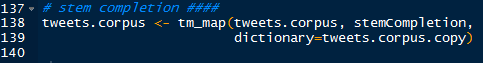Stem Completion Function

Then we can call the function to print out the tweets for 4 through 9 again, and the output for before and after stem completion are stacked below:

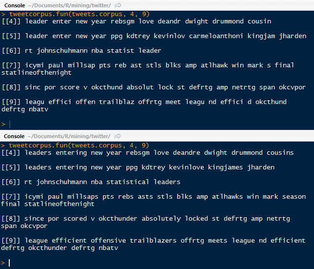Text Corpus Stem Completion Comparison

There are several things to note. Starting at the beginning of tweet 4, we can see that 'leader' was replaced with 'leaders', 'enter' with 'entering', 'deandr' with 'deandre' (DeAndre Jordan the center for the Los Angeles Clippers), 'cousin' with 'cousins' (DeMarcus Cousins, the center for the Sacramento Kings).

However, there are some major differences, such as 'carmeloanthoni' being completely omitted after the stem completion (sorry Melo)- although 'kingjam' was replaced with 'kingjames' (congrats LeBron James). 'statist' was completed to 'statistical'. 'millsap' was incorrectly completed to 'millsaps' (correct as Millsap- sorry Paul). Some shorthand was completed as well- 'reb' was completed to 'rebs' for rebounds. Looking at 'effici' it was completed to 'efficient'.

From the last tweet (9), we see that 'd' was completed to 'defrtg' (short for defensive rating), although that it was just a regular 'd' to begin with. The 'okcthund' was completed to a more familiar 'okcthunder' (Oklahoma City Thunder).

So not all completions did a phenomenal job. That is to be expected when we use the default of completing the stemmed matches with the highest frequency in the dictionary, the copy of the corpus.

Building a Term-Document Matrix

Now that we have stemmed and completed our text corpus, we can proceed to build a term-document matrix. Load the tm and twitteR packages, and continue using the stem completed corpus.

Loading Packages and Text Corpus

In a term document matrix, the terms are the rows and the documents are in the columns. We can also create a document term matrix, and that would simply be the transpose of the term document matrix- the documents are represented by the rows and the terms by the columns. With the TermDocumentMatrix() function, we can create the term document matrix from our tweet text corpus. See in the output below, that there are 606 terms and 186 documents (tweets).

Using the TermDocumentMatrix() Function

There is also a 98% sparsity, which means that 98% of the entries are 0, so the row term does not exist in a particular document column. We can display the terms by calling the term dimension names. It is quite extensive a only a fraction of the 606 terms is show below.

Terms

Observe some (basketball) recognizable terms such as "careerhigh", " blakegriffin", or "chicagobulls"- but which term had the most occurrences in all the tweet documents? We can figure that out using the apply() function and summing across the rows of the term document.

Most Occurring Term: games, 79 times

We can also tweak the function to show the terms with more than 20 occurrences by passing it through the which() function.

Terms With 20 + Occurrences

See that some of the top terms are "asts" assists, "fg" field goals, "games", "okcthunder" Oklahoma City Thunder, and "ppg" points per game among the various terms.

Let us visualize the term document matrix for specific terms and documents. We can assign the occurrences of the most frequent term, "games" in an index, and the following few terms for specific tweet documents. Again, we will use the inspect() function to gain snippets of the term document matrix.

Term Frequencies in Tweet Documents 60 to 70

Note that the sparsity is 87%, so like the rest of the matrix, this sub-matrix is mostly comprised of zero entries. Looking at the frequent "games" term, we do see that particular term appearing in the documents quite often, and even twice in tweet document 64. The abbreviation "gms" is also shown as well.



At the beginning we started with a corpus of tweet text, and we stemmed it, completed the stems, and converted it into a term document matrix. From the TD matrix we were able to count the frequencies of the terms in each document, bringing the data a final step closer to analysis-ready. 

In the next post we will begin to analyze the text data, and we shall demonstrate term frequencies, term associations, and word clouds. Stay tuned!



Thanks for reading,


Wayne
@beyondvalence
LinkedIn

Text Mining: 2. Converting Tweet Text List into a Document Corpus with Transformations Using R

Welcome Back Readers,



Last time in the Text Mining Series we discussed how to retrieve tweets from the Twitter API with the twitteR package in R. Now that we have the text data to work with, we can now transform the text from their raw format into a corpus, which is a collection of text documents.

This post continues from where we left off in Text Mining 1. Read Text Mining 3 here. We require the packages: tm for text mining and SnowballC for word stemming to collapse words.

Now is a good time to download and load them in R- so let us get started! 

Data.Frame to Corpus

As we saw from last time, the raw text in the tweet list object was far from polished and would take some formatting to clean. We start with converting the tweet list object into a data.frame after we load the packages and set the working directory:

Tweet List Object into Data.Frame Object

As we can see, the dimensions of the tweets data.frame has 186 rows and 16 columns. The descriptions for each column are shown below:

Tweet Data.Frame Column Structure

We have columns for the tweet text, whether the tweet is favorited by the user (my account since my app accessed it), how many favorites if any, tweet ID, and so on. Note at the bottom, there are yes/no for longitude and latitude coordinates- so we can track the location where the tweet was sent.

Now that the data exists as a data.frame, we can convert it into a corpus using the Corpus() function from the tm package (the link opens to a pdf of the tm package).

Tweets into Corpus

Observe that the corpus list has 186 text documents, which means that the conversion process converted each tweet into a text document. 

Next, we will transform the tweet corpus and the getTransformations() function displays the text transformations available for the tm_map() function in the text mining package. We have various transformations at our disposal, such as removing punctuation and removing numbers, words, and white space.

Transforming Text

First we will perform the following modifications using the tm_map() function: lowering character case, removing punctuation, removing numbers, and removing URLs. These are completed using the respective commands: tolower, removePunctuation, removeNumbers, and a regular expression substitution using gsub().

Removing Case, Punctuation, Numbers and URLs

The gsub() function allows us to replace the regular expression for an URL link, "http[[:alum:]]*" with "", a non-space for removal. Then we pass that function to the tm_map().

Adding and Removing Stopwords

Next we add stopwords. They are words that are ignored from searches with specific relevant topics and keyword combinations, increase the 'content' of the the tweet, and efficiency of analysis. They include, a, the, for, from, who, about, what, when, where, and more, depending on the analysis. Common stopwords, some even from Google Search filters out can be found here.

We can observe the changes of the text transformation, when we look at a random tweet. Say tweet #4 below. Note how all the punctuation was removed, as with the numbers, and newline escapes "\n", and that all characters are lowercase.

Tweet 4 Before and After

Next time around we shall discuss stemming the documents in the corpus we created and transformed in this post. Stemming involves cutting words shorter to retrieve their radicals. That way we can count their frequency despite the word being spelled differently or being used in a different tense. For example- updated, updating, update are 'stemmed' to updat.

And that is for next time! So stay tuned!


Thanks for reading,


Wayne
@beyondvalence
LinkedIn